In this article, we look at the relationships between frequency, the unit Hertz and order tracking. The most common form of digitising data is to use a regular time-based method. Data is sampled at a constant rate specified as a number of samples/second. The Nyquist frequency, fN, is defined such that fN = SampleRate/2. As discussed elsewhere, Shannon’s Sampling Theorem tells us that if the signal we are sampling is band limited so that all the information is at frequencies less than fN then we are alias free and have a valid digitised signal. Furthermore, the theorem assures us that we have all the available information on the signal.
If we Fourier Analyse a signal, x(t), then we get its components expressed at frequencies measured in Hz. This is completely reversible. That is if we have x(t) we can get X(f). Similarly if we have X(f) we can get back to x(t). This is sometimes written in the form
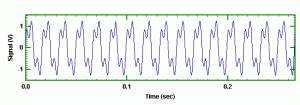
As a simple example consider a test signal composed of two sinewaves. The first one had an amplitude of 1.0, a frequency of 60Hz and a 0° phase. The second one had an amplitude of 0.5, a frequency of 180Hz and a 45° phase. In this example we will sample at 2048 samples/second and acquire 2 seconds of data. The choice of 2048 samples/second is to ensure it exactly matches an FFT size. This is not necessary but it avoids any discussion on end effects. A section of the signal is shown in Figure 1 below.
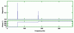
If we FFT this composite signal then we get the modulus and phase plot as shown below.
As expected the amplitudes are 0.5 and 0.25 respectively – recall that the DATS software gives half amplitudes. In the phase plot there is a 270° phase change at 60 Hz and a 45° phase change (270° to 315° ) at 180 Hz. Clearly the 45° phase change is as expected but why the 270° change? Surely it should be 0° and 45° not 270° and 315° . The reason is because Fourier analysis uses cosines and sines with the cosine, not the sine, for the real part. A sine has a -90° or +270° shift relative to a cosine. In other words the basis is a cosine wave not a sine!
All of the above is fairly basic signal analysis. Now suppose we have a rotating shaft and we are measuring the vibrations of the shaft. The nature of the rotating items is that the vibrations occur at multiples and submultiples of the rotational speed. For example if the shaft is rotating at 3600rpm, which is 60 Hz, then we would expect to see responses at multiples of this frequency. These multiples are the orders (or harmonics in musical terms). First order is a frequency which is the same as the shaft rotational speed. In our example this is 60 Hz. The third order would be 3 * 60 = 180 Hz. The general relationship between the order, OR, the shaft speed, R, in rpm, and the frequency, f, in Hz is
Why use order tracking? The reason is of course that the order remains constant with shaft speed; first order is always at the shaft speed; second order is always twice shaft speed and so on. This means we can step into the rotation and it is as if we were moving with the shaft. Instead of sampling at equal increments of time we sample at equal increments of rotation. This is called synchronous sampling; we have synchronised our sampling with the shaft rotational speed. Suppose we had a toothed wheel fixed to the shaft. Instead of a clock providing the command pulses to drive the analogue to digital converter then pulses from each gear tooth will give us equi angular or synchronous sampling at P samples/rev.
We now have data which is sampled in units of a fraction of a rev rather than as a fraction of a second. If we Fourier transform this data we again get a measurement as a function of a frequency type scale but now it is in increments of Orders not Hz. The result is that we now have a signal which gives the modulus and phase as a function of Orders rather than as a function of Hz.
We do not have to sample synchronously to get orders because we can use the relationship between frequency in Hz, f, order number, OR, and rotational speed, R. The procedure is then to FFT the time history, and by using the rotational speed to convert the frequency in Hz to a ‘frequency’ in Orders. This is in principle fine for a constant speed but if the speed is changing over the length of the FFT we have an incorrect result. Also it is unlikely that the frequencies in Hz will map exactly onto integer values in Orders. This means then grouping several order lines to form an rms value.
Thus in dealing with signals from rotating machinery synchronous sampling is preferable but regrettably carrying to synchronous sampling is difficult in practice. It is impossible to sample synchronously with some data acquisition equipment, in particular those with sigma-delta type ADCs must sample at regular time steps. Successive approximation ADCs as used in the Prosig DATS hardware do not have this restriction. This however is not always of practical significance as usually it is difficult enough to get a reliable once/rev tacho pulse let alone N pulses per rev.
The solution is to use signal processing to digitally resample the data. Again we note the implication of Shannon’s Sampling Theorem that if we sample at least twice as fast as the highest frequency present then we have all the information about the signal. With the correct signal processing algorithms we can then resample the initial equi speed time increment data into equi spaced angle increment data. We will not go into this theory and the relevant equations here except to note that the resampling is based on the (sin x/x) function, which is called appropriately a sinc function. This resampling algorithm can be used just to change the sampling rate from say 20000 samples/second to 44100 samples/second for sound replay. When being used for resampling to achieve equal angle it is clear that a once per rev tacho signal is also required. This provides the relationship between time and the total ‘angle’ travelled.
The DATS module ATOSYNC uses a once per rev tacho to convert a regular time series to a synchronous time series. To illustrate its use we will resample the mixed sinewave signal used earlier. A tacho signal which matched the 60 Hz component was used, that is first order will correspond to the 60 Hz signal. Thirty two points/rev were used. A section of the new synchronous signal is shown in Figure 3 below. It looks identical to the original regular time sampled data except that the x axis is now in terms of the total angular distance travelled in Revs.
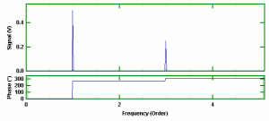
The FFT of the synchronous signal is shown below
This is identical, as expected, to the FFT of the original time history except that the x axis is now marked with units of Orders, not Hz. The two responses are at exactly one and three orders as expected. The mathematics has not changed, just the interpretation and our frame of reference.
As a further observation sampling is sometimes carried out as a function of distance. For example a vibrating beam could be measured at equispaced points along the beam at one instant in time. The increment is then in steps of metres. If we Fourier transformed that signal then we would have a frequency axis in units of wavelength. This option however is not available in DATS.
The more complex signal shown below comes from a steady state run on a vehicle. There is clearly some beating going on. The vehicle speed was not constant so if one analysed in the time domain the amplitudes would be ‘smeared’ over several frequencies.
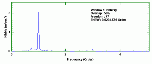
Figure 6 below shows the Order tracking analysis where it is quite clear that the energy is mostly at first order with some side bands and also some small contributions in the second and third orders.
An even more revealing signal is to analyse a simple swept sinewave such as shown below.
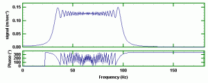
If we analyse this as a standard time history we get the expected spectrum from 30 Hz to 100 Hz as shown in Figure 8.
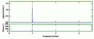
Now if we synchronously sample the swept sine using itself as its own once/rev signal and frequency analyse then we get the synchronous signal as shown in Figure 9.
The entire signal is now concentrated entirely at the first order. The amplitude is the half amplitude and the phase jump is 270° . If we look at the synchronously sampled signal, which is shown in Figure 10, then the ‘swept sinewave’ is now just a ‘constant sinewave’. We have a constant number of points per revolution and all evidence of the change in speed has gone.
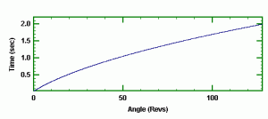
The software does however retain the time versus angle travelled data in another signal so that in practice no information is lost. This is shown below in Figure 11.
Because the rate of change of speed was a constant, then the time vs angle travelled curve is of the form time = k*sqrt(angle).
Dr Colin Mercer
Latest posts by Dr Colin Mercer (see all)
- Data Smoothing : RC Filtering And Exponential Averaging - January 30, 2024
- Measure Vibration – Should we use Acceleration, Velocity or Displacement? - July 4, 2023
- Is That Tone Significant? – The Prominence Ratio - September 18, 2013







dear sir will you please help me out to find out the peak values for a particular order(i.e 2nd order) i mean to say a formula. when i have angular acceleration and engine speed as a raw data.
thank you
Pingback: What's the Story Behind Unit Hertz in High Tech Tools? | EducationNews