
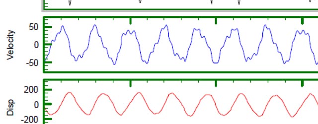
Accelerometers are robust, simple to use and readily available transducers. Measuring velocity and displacement directly is not simple. In a laboratory test rig we could use one of the modern potentiometer or LVDT transducers to measure absolute displacement directly as static reference points are available. But on a moving vehicle this is not possible.
More here… OmegaArithmetic.pdf
The following two tabs change content below.

Dr Colin Mercer
Founder / Chief Signal Processing Analyst (Retired) at Prosig
Dr Colin Mercer was formerly at the Institute of Sound and Vibration Research (ISVR), University of Southampton where he founded the Data Analysis Centre. He then went on to found Prosig in 1977. Colin was MD and Chairman of Prosig for many years. He retired as Chief Signal Processing Analyst at Prosig in December 2016. He is a Chartered Engineer and a Fellow of the British Computer Society.
Latest posts by Dr Colin Mercer (see all)
- Data Smoothing : RC Filtering And Exponential Averaging - January 30, 2024
- Measure Vibration – Should we use Acceleration, Velocity or Displacement? - July 4, 2023
- Is That Tone Significant? – The Prominence Ratio - September 18, 2013


Dear Dr Mercer:
I read your article about Omega Arithmatic and try to apply it on my experiment results, and met some problems really need your help!! I use accelerometer to collect data. Following the article, I do the Fourier transform and divided by -w^2 to get the displacement spectrum. After that when i do the inverse Fourier transform to get displacement time sequence, the result is a “complex vector”. So my question is how can I convert this “complex vector” to a displacement time sequence?? Is it correct to get the magnitude of each complex number, or just keep the real part and leave the imaginary part?? I really appreciate your kindly help!!
Hi Linus,
Did things work for you ? I tried the same method but data doesnt agree with physical event.
Thanks!
must do the complex calculation, use both parts. u can only use the multiplicaion and addition, basic calculation rules are:
(a+jb)*(c+jd) = a*c-b*d + j(a*d+b*c); (a+jb) + (c+jd) = (a+c) + j(b+d);
if use c, u can use two arrays to hold the real part and imaginary part separately, input spectrum vactors are acc_real[N], acc_imagine[N], N is the number of vectors.
in yr programm what u only need to calculate are: omega_disp_real[N], omega_disp_imagine[N].
Omega_disp_factor_real = -1.0/w^2; Omega_disp_factor_imagine = 0;
for each n
omega_disp_real[n] = acc_real[n]*Omega_disp_factor_real – acc_imagine[n]*Omega_disp_factor_imagine + acc_real[n]*Omega_disp_factor_imagine + acc_imagine[n]*Omega_disp_factor_real ;
omega_disp_imagine[n] = acc_real[n]*Omega_disp_factor_real – acc_imagine[n]*Omega_disp_factor_imagine;
omega_disp_real[n] = acc_real[n]*Omega_disp_factor_imagine + acc_imagine[n]*Omega_disp_factor_real ;
time squence magitude value use: magitude_disp[n] = sqrtf(omega_disp_real[n]^2 + omega_disp_imagine[n]^2); phase[n]=…
if use matlab, the vectors can be directly devided by -w^2, Omega_disp = acc_fft_vector./(-w^2).
matlab takes care of the complex calculation automatically.
time squence magitude value use magitude_disp = |Omega_disp|; phase value: …
In case of simple acceleration signal like sin(w*t), the displacement signal is displacement=IFFT(FFT(sin(w*t)/(-w^2))). It works well and good for this.
D.I (sin(w*t)) = -sin(w*t)/w^2 = IFFT(FFT(sin(w*t)/(-w^2)))
D.I. –> double integration
But however in case of composite signals with sinusoids of different frequencies and amplitudes what is the dividing factor.
D.I (sin(w*t)+sin(2*w*t)) = -(sin(w*t)/w^2)-(sin(2*w*t)/(2*w)^2)
is not equal to IFFT(FFT((sin(w*t) )+sin(2*w*t))/(-w^2)))
Sudakhar
You divide each X(f) by its own frequency f (actually divide by -[2*PI*k*df]^2)
However be careful to avoid division by zero at start – this is the dc component so set it to zero. Low frequencies are a pain as we get the so called 1/f noise – I option ignore any frequencies below 1Hz and force the to zero
Linus
The FFT and its inverse deal in complex numbers. In this sense your measured accelerations signal is the real part of a complex signal with zeroes for the imaginary part. Strictly speaking a Full FFT will give you a frequency spectrum from -half sampling rate to +half sampling rate but when we have real only data then the FFT values for the negative frequencies and the positive frequencies are related. Specifically X(-f) = conj{X(f)} that is if X(f)= a+ib then X(-f)= a-ib. In a digital representation for a real signal we have X(N-k) = conj{X(k)}.
What you get precisely when you do the FFT depends on your software package. What you need is software that has a real part only FFT which produces the usual half range result (zero to sample rate /2) and a half range Inverse FFT. This latter algorithm is often not available (it is in DATS of course!).
If you do not have the relevant inverse then
do the forward FFT of real data
divide real and imaginary parts by -(omega^2)
generate the x(N-k) complex values from conj{X(n)}
do full range inverse FFT
If done correctly you will find that the imaginary part of the inverse transform is effectively zero. You need to be very careful with the scaling. If the time between samples was dT and you have N acceleration values (N is power of two) then your frequency spacing df = 1/NdT and the value of omega for X(k) is 2*PI*k*df.
Dear Mercer,
I first transform my time series data to f domain using fft matlab command.
fftX = fft(Ax,L); %L=number of samples which is 2048
fftY = fft(Ay,L);
fftZ = fft(Az,L);
And find the displacement matrix for frequency vector ‘f’ of 0 to SamplingRate ‘fs’/2.
df=fs/L; %where df=frequency spacing, fs=sampling rate
for j=2:L/2+1 %Consider half range
omega(j)=2*pi*f(1,j)*df;
velocityX(1,j)=fftX(j,1)./(1i*omega(j));
displacementX(1,j)=fftX(j,1)./(-1*omega(j)^2);
end
omegaVX(1,1)=0;% To avoid division by zero at start – this is the dc component so set it to zero.
omegaDX(1,1)=0;
After getting velocityX and displacementX vectors, I changed velocityX and displacementX vectors to full range by conjugating to perform full range IFFT.
%change to full range by conjucating
for j=1:sizeOmegaX-2
secondVRange(j)=conj(omegaVX(1,sizeOmegaX-j));
secondDRange(j)=conj(omegaDX(1,sizeOmegaX-j));
end
omegaVX(1,1026:2048)=secondVRange;%full range
omegaDX(1,1026:2048)=secondDRange;%full range
And then, ifft them.
velocity=ifft(velocityX);
displacement=ifft(displacementX);
-When I followed all the above procedures, my velocity vector has immiginary part and displacement vector has only real part. I think I have something wrong with concepts. Your kind help is highly appreciated.
Best regards,
Nyein
Hi
I missed this so apologies for very late reply. Yes the velocity should be in the imaginary part with real part as practically zero. This is because velocity is 90 deg phase shifted with regard to accel. Similarly the displacement should be in the real part with effectively zero imag part as it is phase shifted by 180 deg. Basic relationships are [velocity = Accel/(i*omega) = -i*Accel/omega] and [disp = -Accel/(omega^2)] .
Colin
I’ve seen in training literature the statement about integration from acceleration to velocity ‘ The process involves a phase shift that supresses the higher frequency information and amplifies the lower frequency information.’ Your Omega Arithmatic article does stress the phase shift importance but does not directly confirm the statement. could you please share your comments about the relationship between phase shift and integration and the effects on the frequecy spectrum?
Integrating from acceleration to velocity, or from velocity to displacemerit, involves a 90 degree phase shift. If we integrate directly from acceleration to displacement then of course there is a 180 degree phase shift. None of these phase shifts is anything whatsoever to do with suppressing the higher frequencies. The amplitude change comes about because we are dividing by the frequency in radians/sec, usually called omega (=2 * PI * frequency). So we get the amplitude change at higher frequencies simply because the frequency is larger.
We are actually dividing by (2 * PI * i * frequency) , the ‘i’ causes the phase change and the (2 * PI * frequency) changes the amplitude. If you can bear a little maths suppose we have an acceleration spectrum A(f) with phase Theta(f). Now if R(f) is the real part and I(f) is the imaginary part then we know
A(f) = Sqrt {R(f)**2 + I(f)**2} and Theta(f) = arctan{I(f)/R(f)}
Now let us divide the read and imaginary components by (i*Omega), which is like multiplying by [1/(i*Omega)] = [-i/Omega].
Velocity Spectrum = Acceleration Spectrum * [-i/Omega]
= [R(f) + iI(f)] * [-i/Omega]
= [-i*R(f)/Omega] + [I(f)/Omega]
So the Real part is now [I(f)/Omega] and the
imaginary part is [-R(f)/Omega]
Hence the Amplitude of the Velocity Spectrum, V(f), is given by
V(f) = Sqrt{[I(f)/Omega]**2 + [-R(f)/Omega]**2}
= Sqrt {I(f)**2 + R(f)**2} / Omega
= A(f) / Omega
The velocity phase, say Phi(f), is given by
Phi(f) = arctan{[-R(f)/Omega] / [I(f)/Omega]}
= arctan{-R(f) / I(f)}
= Theta(f) – PI/2
This last relationship is not intuitive but if you do some simple geometric drawings then you can see the result.
Dear Dr. Colin Mercer
Your article Omega arithmetic is very interesting for me. I use for statistical analysis my signals (random vibration of trailer wheel from road) software Microsoft Excel (mean, standard deviation, histogram, kurtosis, skewness, FFT, …) . I measured accelerations (time domain) , I do id FFT transform (Excel can make FFT only for maximum 4096 values) and I received real and imaginary parts, then I divided each part with –omega2. I created from first 2048 values the complex values and I do it inverse FFT from 4096 parts but my Displacement has real and imaginary parts and in this point I need your help because my imaginary parts are not effectively zero. I don’t know if you know FFT in Excel.
Thank you very much for your help. I don’t know if Microsoft Excel is good software for omega arithmetic, but I will try to do it with Excel.
Excel would not be my first choice for frequency analysis! Before discussing the actual FFT in Excel, it is worth noting that doing an FFT of a random signal still has the same degree of randomness. That is there is no averaging involved.
I have looked at Excel FFT and it is a basic full range FFT.That is it computes from zero Hz to sample rate , not sample rate/2. The upper half is the complex conjugate mirror about the Nyquist frequency (sample rate/2) of the lower half. The actual frequency values you need to multiply by are for the finite half from zero to Nyquist. The frequency after to Nyquist is (Nyquist-frequency increment) and so on until you get down to (frequency increment).
For example suppose you had a sample rate of 512 samples/sec & you used a 64 point FFT then your frequency increment is 8 Hz(Sample rate / FFTsize). The frequencies then rise from 0 to 256 in steps of 8 , then as 248,240 to 8. This is because the FFF is not computing from zero to sample rate but from -Nyquist to +Nyquist. Its just the way that the FFT is implemented.
Note also that you need to divide the Excel FFT by the FFT size to correctly get to half amplitude. This can be done when you make the final time series. I do have a simple Excel Spread sheet example from displacement to velocity.
Dr. Mercer can you please email me the spreadsheet so that I will understand better ? I have already sent email to prosig.
Thanks!
Dear Dr. Colin Mercer
Thank you very much for your answer. I sent today email to prosigusa@prosig.com with request, that my email with short example will be send directly to you.
Hi Colin,
The .pdf was very interesting, thank you for providing this resource. I have a question:
“We are actually dividing by (2 * PI * i * frequency) , the ‘i’ causes the phase change and the (2 * PI * frequency) changes the amplitude.”
Could you explain how to create this “frequency” vector? Normally, after taking a fft in Matlab, if I want to plot Velocity Amplitude vs. freq (Hz), I create a vector from 0 to #datapoints/2, then divide this vector by the length of the sample in seconds. The result is the frequency axis in (HZ).
Is a similar method used to create the frequency vector for use in Omega Arithmetic?
Thus far, my attempts to convert velocity to displacement are not working on my sine wave test signals. The phase change of the result is correct, but when I change the frequency of the velocity, the amplitude of the displacement result remains the same. Therefore I think there must be something wrong wtih my frequency vector.
Thanks for any advice,
Mark
Mark
You basically construct the frequency vector as you did for your frequency axis, together of course with the 2*pi. In principle you have to make it complex with a zero real part. Now, there is a twist, which depends on the type of FFT you do. That is, do you have a full range (0 to sample rate) or a half range FFT (0 to sample rate/2). Sample rate/2 is often called the Nyquist frequency. Also of course you want it in Real and Imaginary form.
The way you actually construct the frequency vector is similar to described in the Excel notes above.
Because of the interest l will add a Part 2 article.
Colin,
I look forward to part 2.
Matlab takes a full range FFT, as in you can see the mirror image of the data and only end up using half of it to make a regular FFT plot.
I am not having trouble constructing the positive half of the frequency vector (I don’t think) because my regular FFT plots work fine using the same method.
Per your advice I’ve tried to construct the entire frequency vector, including the negative frequencies, by mirroring my positive frequencies. But, I must have a small problem somewhere. After the omega arithmetic operation where I divide by (2*pi*freqvector*1i), most of the result’s elements are in the form xReal+Yimaginary. But, the first element is -Inf, and the last element is Inf + i*Inf.
I’ll work on it some more tomorrow…
It turns out that you can’t do an IFFT of Infinity. Changing all INF’s to 1’s got the process working.
A simple fix but I thought I’d share in case someone runs into this in the future.
Dear Dr. Colin Mercer
Thank you very much for the PDF, it was really helpful
I tried to implement whats in the PDF in Matlab to integrate a sin signal only single integration and it worked perfect match with the theoritcal integration of sin.
But when the input signal was like y = [zeros(1,16) ones(1,16)] the integrated signal wasnt as expected. the shape of the signal looks OK but the integrated values didnt look like 0000..00 12345…16 for delta T of 1 .but it was like
4.3102 4.2200 4.2699 4.2348 4.2626 ……….. 15.7626 16.7348 17.7699 18.7200 19.8102
I wonder where did this ~ 4.3102 came from? the integration should look like
0000..00 12345…16
Below is the implementation code of your idea in Matalb.
Thank you very Much !
n=32 %samples/period
delta_t = 1 %// sampling time
f=1/(delta_t*n)
periodTime = 1/f
t=0:delta_t:periodTime-delta_t; %input one period to the FFT
N=length(t)
df=1/(delta_t*N)
%this signal integration didnt work
y = [zeros(1,16) ones(1,16) ]
% below signal integration works great (commented)
%y = sin(2*pi*f*t);
% insert zero mean signal to the FFT
meanY = mean(y);
y = y – mean(y);
% construct OMEGA
for i=1:1:N/2+1
omega(i+1)=i;
end
omega(N/2+1)= 1;
for i=N/2+2:1:N
omega(i)=-(N-i+1);
end
omega(1)= 1;
omega = 2*pi*df*omega ;
trans = fft(y);
%devide each frequency by jomega
FD = trans./(j*omega);
integrated = ifft(FD) +meanY*(t+delta_t)
%theoryINT = -1*cos(2*pi*f*t)/(2*pi*f);
%plot( t,theoryINT,’-*r’,t,integrated,’-og’)
plot( t,integrated,’-O’)
Dear Dr. Colin Mercer,
Your article is very interesting and I can found some responses for my problem. In fact, I’m civil engineering and I work in a project that the principal goal it’s the road impact measurement So, to describe the impact, i measured the acceleration for each shock to obtain the road displacement. In this moment, the data processing was making in the time domain (double acceleration integration). After a baseline correction, i can obtain the signal almost correct.
I was reading about the acceleration “frequency integration” by the FFT. The problem: i work with excel. So, i need your help, I’m very interesting to obtain a copy of your excel spreadsheet to obtain the displacement by acceleration spectrum integration, because I’ve (Like Mr. Jozef Steinhubl, I get a real part and an imaginary) some problems to obtain the displacement with my spreadsheet in excel.
Thank you very much for your help.
Best regards,
Miguel Angel BENZ NAVARRETE
So, i read about the acceleration “frequency integration” by the FFT. The probleme : i work with excel. So, i nedd your help, ’cause i’m very interesting to obtain a copy of your excel spreadsheet to obtain the displacement by acceleration sprectum integration , because i’ve somes problems to obtain the displacement with my spreadsheet in excel.
Thank you very much for your help.
Dear Miguel Angel BENZ NAVARRETE
I solved the problem of FFT integration with excel. If you are interesting send me email on steinhubl.jozef@gmail.com, I can send you my excel program.
Best regards
Steinhübl
Dear Mr. Steinhubl Jozef,
I’m interesting and I will sent you an e-amil,
Je vous remercie par votre aide.
Best regards,
Miguel Angel
Dear Dr. Colin,
Please, forgive my poor English.
I’m just trying to introduce myself into FFT calculations and I have an elementary question to you.
As an example, suppose I have a time history of velocities signals (after integration of accelerations) and I take a FFT of these signals, say, up to the Nyquist frequency.
The real parts of my imaginary vector will return to me the amplitudes and the imaginary ones will return me the phases. So now, I will have the amplitudes related with the several frequencies. However, I would like to know how to obtain the transformation of these amplitudes in terms of my field (primary) variable, that is, in terms of velocities, so that I can get the spectrum in terms of velocities. In this case It will be possible to perform inverse FFTs for single values, that is for each frequency of the spectrum?
Thanks,
Luiz Eduardo
Hi Dr Colin, i want to ask if my accelerometer receives the data as show below in 3 axis, how to compute them into displacement and velocity?
Accel: 0.260530680418,-0.790787398815,-0.553876399994
Accel: -0.177965387702,-0.922816634178,-0.341669201851
Accel: 0.215337008238,-0.945518255234,-0.244182661176
Thanks,
Kelvin
Dear Dr.Colin Mercer,
I am trying to make a vibration sensor to measure vibration of washing machine during spin cycle with a MEMS accelerometer and arduino to collect the acceleration data. I will be processing the data using MATLAB.
I went through your comments and I want to know if the FFT method you suggested works at a steady vibrations or even with varing disturbing frequencies.
I ask this because I have to measure the displacement at resonant frequency of washing machine but for safety of the machine this speed is passed very fast. The resonance occurs at about 200rpm while the machine goes from 95 to 400 rpm in 15 s. Will the measurement at this zone and omega arithmatic procedure you explained serve my purpose??
close all,clear all,clc
%a=xlsread(‘m1vt.xlsx’,2);%,2,choose 1 after’ is read pg 2
%a=xlsread(‘free-radial direction.xlsx’,3);
%v=a(:,2);
%t=a(:,1);
t = 0:0.01:1;
%v =20*sin(2*3.1415*5*t)
Dear Dr.Colin Mercer:
I try your method to convert velocity to displacement
using a simple signal and compare to those obtained from direct integration methid. It shows difference. The following is my matlab code. Can you help me on this.
t = 0:0.01:1;
v=3*sin(4*2*pi*t) + 5*sin(2*2*pi*t);
plot(t,v);%velocity
dt = t(2)-t(1);
N = length(v)-1;
v_fft = fft(v);
f = (0:N)/(N*dt);
df=1/N/dt;
i=sqrt(-1);

for k=1:N+1;

d_fft(k)=v_fft(k)/(2*pi*k*i*df);

end

cy = real(ifft(d_fft));%displacement
total_t=1/df;
T=total_t*(0:N-1)/N;
figure,plot(T(1:N/2),cy(1:N/2));
%checker :displacement by direct integration
for t=1:1:101;
D(t)=-3*cos(8*pi*t/100)/8/pi-5*cos(4*pi*t/100)/4/pi;
end
figure,plot(T(1:N/2),cy(1:N/2));
hold on
plot(T(1:N/2),D(1:N/2),’r’);
Anna
I have not looked in detail at your matlab code but I think that the error comes in the section
i=sqrt(-1);
for k=1:N+1;
d_fft(k)=v_fft(k)/(2*pi*k*i*df);
end
cy = real(ifft(d_fft));%displacement
Also as a minor observation it would be clearer if you used df=1/(N*dt); rather than df=1/N/dt;
You have assumed as so many people do that the frequency range of the resultant FFT goes from zero to (N-1)*df. That is not the case actually as the frequency range covers the region from -[Nyquist/2] to +[Nyquist/2], but in the software in most FFT algorithms arrange the results from 0 to +[Nyquist/2] in the first half followed by frequencies from -{[Nyquist/2] – df} to -df. Thus you need to split your loop into two loops with the first one handing the positive frequencies and the second one handling the negative frequencies.
I think you may also be dividing by the wrong frequency anyway as the first frequency is at zero Hz. This needs special handling obviously to avoid the division by zero. Clearly we are only interested in the non zero frequencies so you first have to reduce the input signal to a zero mean. This will result, theoretically, in a zero amplitude component at zero Hz, but you need to force that to be zero and not rely on the arithmetic carried out by the software. If you do the math the limit case by L’Hospitals Rule is zero.
The very low frequency end by the FFT method is susceptible to error because of the division by k*df when df is small such that k*df<1 as in that region any errors are magnified. Conversely that is the region where direct integration is the most accurate. So in the real world when needing integration, I use both approaches dependant on the frequency range of interest. Also you need to pay attention to the direct integration method you use. Odd order integrators are hopeless above Nyquist/4 – at Nyquist/2 they have a zero magnitude tranfer function. Also good even order integrators incur a time delay. See my notes at
https://blog.prosig.com/2012/06/15/wide-band-integrators-what-are-they/
Colin
Anna, please consider for each value of frequency obtained with your analysis program:
a -For each specific frequency, perform an inverse FFT (IFFT) in order to recover your primary variable, that is, the velocity related with the frequency considered;
b – Now, divide the velocity by Omega=( 2.PI.f) to find d(f), that is: d(f) = v(f) / ( 2. PI. f );
c – If you intend to work with accelerations directly, for each frequency considered perform IFFT to get A(f) and then calculate: d(f)=A(f)/ (2. PI^2 . f)
Dr. Collin explained this in other articles.
Also, take a look at:
http://www.cbmapps.com/docs/28
(Conversion Formulas)
Regards,
Luiz Eduardo
Dear Dr. Collin,
Thank you for sharing this great tool. I have a question regarding the method, though:
I am able to convert from Acceleration to Displacement following the equations and domain transformations. However I am not able to do the same backwards (convert from Displacement to Acceleration).
I am using Matlab for the FFT and the IFFT; I am sure that the data in frequency domain is correct. I think that my problem is returning from frequency domain to time domain (using the IFFT function). Is there something I should take a look while doing the inverse transformation?
Thank you for the help you can bring. And thanks again for the method; it has been really helpful.
Regards,
Agustin
Dear Dr. Colin,
First of all, Many thanks for your article and the continuous reply it is very useful for the students like me and much appreciated your time and the dedication through out your busy schedule. I have a couple of things to clarify from you about Omega arithmetic method, I would much appreciate if you could help me with this:
I am currently doing some experimental modal analysis using impact hammer test and I do have the impact force and the response acceleration time histories, I need to retrieve the displacement time history from the measured acceleration time histories.
Firstly I have tried with the time domain method using MATLAB but it couldn’t give me promising result since I didn’t have high sampling resolution during my measurements, and currently I have gone through your article about Omega arithmetic method and have implemented in MATLAB, the result was little promising but the DC component of the retrieved displacement was Ofsted from the measured acceleration time histories, and I am suspecting on the following things, could you please kindly help me if possible to tackle the problem:
1. I am doing full scale fft of the measured acceleration in MATLAB, and dividing this fft by -Omega^2, where my Omega is calculated as follows:
outincr = srate / fftlen
where, srate- sampling rate and fftlen- length of fft.
outlen = length of ‘fft’
outlimit = ( outlen – 1 ) * outincr
f = ( 0 : outincr : outlimit )
Omega= 2*pi*f
Could you please kindly guide me whether I am calculation the Omega in right way or not? because I am confusing with the full range fft and the corresponding Nyquist frequency.
2. Since we have zero at the start of the Omega, it is problematic when we divide the fft with -Omega^2. In your previous comment you said we need a special handling, is it OK to add any numerical value at the start of the Omega? for example lets make the starting value of the Omega as 1? if not how we can handle this?
3. And you mentioned that we have to remove or force the DC component of the signal to be zero, do we need to remove the DC component of both the Fourier transformed acceleration signal and the acceleration time history?
I am really sorry for the long message and really sorry to be pain but I really need your help.
Thank You,
Kind Regards,
Thivakar.
Dear Dr. Colin Mercer,
Your article is very interesting and I can found some interesting thinking for my problem. In fact, I’m civil engineering and I work in a project that the principal goal it’s the measurement of sleeper displacement under moving trains. But, I still do not believe that application of this method (Omega arithmetic’s) will be successful, so will be possible to calculate shifts sleepers from measured acceleration. Time acceleration record from sleepers is relatively complex. Do you have any experience in this area? What acceleration sensors would be appropriate? There is an opportunity to try this method in same free software? I think the problem is how to select the signal filtering and sampling frequency and so on. Thank you in advance for your advice. Jaroslav Triste, University of Technology.
Hi
As you are interested in very low frequencies, down to 0Hz I suspect, then this method would not be good. In simple terms the relationship between acceleration and displacement is (Accel = omega^2 * Displacement) where omega is the frequency in (radians/sec) = 2*PI*f with f in Hz. That means we have in effect
(displacement = accel/(omega^2)) so as the frequency approaches zero then the calculated displacement becomes much too high.
So one heeds to ‘ignore’ the very low frequencies, which the software provides for.
This is OK if you are just interested in the vibration response of the sleeper at higher frequencies for resonances that may cause some long term fatigue problem but I doubt that is your concern.
To get the measurements I believe you are seeking you need either an optical transducer or a strain gauge setup is better. The challenges there are getting a reference point. It depends on whether you want the absolute movement of the sleeper or its motion relative to the ground.
Colin
Dear Dr,
Heaps of thanks for this informative blog. I have a bit of confusion in conversion:
We know that (Accel = omega^2 * Displacement); so if we need to retrieve the displacement from acceleration records we would have (Disp= Accel/ omega^2 ).
However,I cannot figure out why in the article (and throughout comments in here) it is mentioned (Disp = -Accel/omega^2) .What is this negative for?
Thanks for your insights
I am unable to download the pdf document. Can anyone share the same?
My email ID is neihguk.david@mahindra.com
Thanks,
David
Hi David. Thanks for spotting the broken link. It should work now. We have also emailed you the PDF.
Hello all,
Can anyone suggest how to perform an FFT/Omega transformation on realtime data to output realtime displacement? Would this be the correct way to do this? How is it done with the realtime vibration software offered by prosig?
Hello all,
I have a question regarding the example of Omega Arithmetic described in the pdf. After trying to recreate the results in the article the only way I was able to get the correct scaling of the inverse FFT result was to scale the original FFT estimate in the following manner:
FFT(X) * ( 3/ length(X) ); where 3/ length(X) = 1.5e -5.
I do not know why this works. All the material I have read about proper scaling of FFT do not mention this kind of scaling. It seems like a very arbitrary value to scale by which tells me I may have made a different mistake elsewhere. Perhaps I miscalculated omega or the frequency spacing. Can anyone offer any suggestion? My calculations done in R language are the following:
total sampling time= 0.2 s
sampling rate= 100,005 htz
total samples= 20,000
time<-seq(1,1.2,0.00001)
acc<-NULL
for(i in 1:length(time)){
acc[i]<- 10*sqrt(2)*sin(2*pi*50*time[i])+5*sqrt(2)*sin(2*pi*120*time[i])
+8*sqrt(2)*sin(2*pi*315*time[i])+2*sqrt(2)*sin(2*pi*500*time[i])
}
df=( length(acc)/ ( max(time)- min(time) ) )
freq<-seq( 0, df, df/ length(acc) )
freq<-freq[ -length(freq) ]
accfft<-fft(acc)*(3/length(acc))
plot(freq[1:length(freq)/100],abs(accfft[1:length(accfft)/100]), type = "l")
abline(v=c(50,120,315,500), col="red")
w3<-2*pi*( df/length(acc) )
accOYfft<-NULL
for( i in 1:length(accfft) ){
accOYfft[i]<-(accfft[i])/-(w3*i)^2
}
disp<-fft( accOYfft, inverse = T )
disp<-Re(disp)
plot(time, disp, type = "l", col="blue")
Hello Daniel,
Thank you posting on our blog.
It is very interesting to see you R language code, thank you for sharing.
I am afraid I cannot say I have ever used a statistical analysis language like R before and therefore I could not comment.
Perhaps some of our other readers will have experience using R and may be able to comment in time.
To move forward I could only suggest you consider one of two options, either option A, use a signal processing package like Prosig DATS that provides complete and ready to use tools, rather than having to create your own algorithms or option B use a more common language like C where support from an open source community might be more available.
Thanks again for sharing!
Hello,
Thanks for your advices. I tried these calculations in R because at the time that was the only programing language i knew. I am now using a similar algorithm in python to estimate displacment of an accelerometer in realtime. I got positive results when testing the system, however i find again that I must multiply my final values by a scaling factor for the magnitude or “amplitude” of displacment to be accurate. If my acceleration is input as m/s^2 shouldnt my displacment be output as m? I just want to ask is it normally neccesary to have to scale the final result? Under what circumstances would this be necassary? Is there a good method for estimating the scaling factor?
Hello Daniel,
Thank you for posting back on our blog.
I understand your issue. You are quite correct, if your input acceleration is in m/s/s then the velocity will be in m/s and the displacement will be in m.
There is no scaling factor however, only that you should be aware of the change in units.
There are conversion charts, they are (Y Axis) log of Amplitude and (X Axis) Frequency, these should help you understand if your conversion is taking places correctly.
Good luck.
Hi,
I have the experiment results from PCB instrument acceleration Vs time. I need to find the acceleration to velocity and displacement. kindly help me out this what methods going to be use and analysis. please if you have a code please send to me somudce@gmail.com
Dear Soman
If you download the PDF in the link in the article it explains the technique that you should use. There are also other posts on the subject here… https://blog.prosig.com/2013/07/25/how-do-i-convert-between-acceleration-velocity-displacement/
If you read the comments above there is lots of help.
I am sorry but we don’t have any code that we can share.
Link to the .pdf seems to be broken
Dear SteveG – thanks for spotting that. The PDF has been restored.