The requirement was to develop a ‘standard’ test for assessing vehicle power steering pump noise (and sound quality). Measurements needed to be objective so that the method would be suitable for evaluating dissimilar vehicles and different types of pumps.
Noise is an important consideration when a consumer is selecting a new vehicle. It is, therefore, imperative that every aspect of the vehicle’s acoustic profile is thoroughly understood and refined.
From an end-user point of view, the assessment criterion is simply how much will the driver or passengers hear the pump noise in relation to the vehicle’s background noise. That is, will the pump produce what may be called audible tones with the vehicle in different operating conditions.
For the development engineer, this means finding a suitable measurement setup, selecting vehicle test sequences and deriving an analysis technique that will allow automated tests to be carried out very simply in a vehicle. Obtaining repeatable test results in any automotive testing application is notoriously difficult and this is especially true in noise applications where there are many potential sources of error. Often the engineer has to be innovative in his test method in the quest for repeatable results. Many test and analysis scenarios must be considered before confidence in the selected technique is established. Ease of use, speed of analysis and flexibility are of prime concern when choosing the analysis software. It is also essential that reports are fully automated if results are to be acted on quickly. How many times does one hear that the test was completed, but we are waiting for the results and now we no longer have the vehicle! Employing a good data acquisition system, complete with signal conditioning under software control is also essential to overall speed. Naturally, the system must be portable and must operate in the vehicle.
Waterfall displays are often very revealing and can simplify the identification of resonances and speed-related vibrations
Measuring the noise from the steering pump is complicated by several factors. First, the noise is multi-tonal. It has a lot of background masking and, finally, it is dependent on the engine speed.
The obvious initial measurement setup is to place a microphone in the expected vicinity of the driver’s or passenger’s ear. A refinement would be to use, say, a binaural head to simulate the interference effects of a human being, but as noted later a binaural head was not suitable although more than one microphone is required. The test sequence determines whether the pump will be audible in each operational condition. If it is audible then corrective action will be required. Clearly then the assessment method must also be able to give the engineer sufficient information to allow further diagnosis and treatment if this is necessary. A small, but rather obvious, point is that the data acquisition subsystem and the laptop PC must be very quiet if they are to measure noise.
As previously stated, one of the main requirements was for a simple and repeatable test. For this a stationary engine run-up test with “loaded” steering was chosen. For this the vehicle was stationary and the steering turned to achieve a constant 50 Bar at the pump outlet. To perform the test the engine speed was increased slowly from idle to 3000rpm. [It should be noted that the data shown here was from an early trial test and a truncated 2000rpm test was used.] The Prosig system was configured to monitor the pressures and start/stop automatically at specified engine speeds.
One technique often used in vehicle noise investigations is to cover the offending item with noise absorption materials to see if this makes a measurable difference. The difference between the masked and normal state may then be used as a suitable metric. Whilst there were some differences, these were small and inconclusive. Also, the masking technique is difficult and is prone to error so that approach was considered as impractical outside the research laboratory. Using a direct simple measurement scheme with more signal processing was determined as being the practical way forward.


During the initial phase of the work several tests were carried out with the aim of identifying a ‘standard’ microphone position from which repeatable results could be gathered. Using just a single microphone or two microphones (in a binaural head) proved to be unsatisfactory. Tests proved that even small variations in microphone positioning caused a wide spread in test results. The existence of so called ‘high spots’ and ‘dead spots’ were identified, but individual results were too scattered to give anything conclusive. These are, of course, nodes and antinodes of the acoustic standing waves in the car. When vehicle to vehicle comparisons are also taken into account the single position microphone or binaural head results gave even greater variability.
By using the correct signal-processing techniques assessment of the rms level is determined
It became clear that an array of microphones was required. After several iterations it was found that data from six microphones arranged in a sphere gave reliable results to account for ‘high spot’ and ‘dead spot’ positions. However, only three test runs were needed to average out anomalies and slight variations between runs for a specific vehicle type. This then gave 18 sets of data for one test. An additional advantage of the microphone array is that it extends the evaluation to cater for different driver positions. It might be thought that the analysis technique would be to form a spatial average of all six microphones and then to average over all three runs. As discussed below this was not the approach taken.
Obviously, quick and easy to use acquisition/analysis tools are an essential aid for the engineer during the investigation phase of establishing a test method. A rich variety of interactive analysis tools are essential for ‘what if’ type investigations. Several ideas for an analysis technique were investigated including (but not limited to) such things as averaging results in the frequency domain, but these methods were soon eliminated due to ‘dead spot’ spoiling of results.
In this application, as is many times the case, a significant volume of data needs to be collected and rapidly analyzed before any results are revealed. The raw time histories of all microphone positions look very similar to the eye and it is impossible to draw any conclusions from them. Just determining the overall level also gives no indication. Clearly a frequency based analysis is required. As both the vehicle noise and the pump noise are speed dependent then the essential technique is to use a waterfall analysis. This is quite a simple technique, which relies on simultaneously measuring the speed and the noise signals.
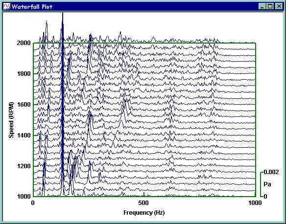
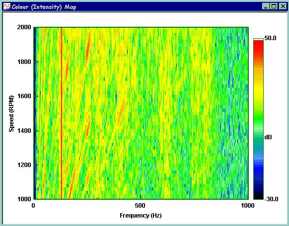
Generally, the speed signal is from a tacho that provides one or more pulses per revolution of the engine or the part being tested. In this case a tacho signal was provided by the pump. The tacho signal is first analyzed to give a speed versus time curve. Short segments of data centered at selected speeds, which are typically every 20 rpm, are then Fourier analyzed and shown as illustrated in Figures 1a and 1b. Note that the FFTs are spaced 40 rpm apart for clarity. The classical method of displaying waterfall data is shown in Figure 1a. The vibration amplitudes are plotted on a linear scale. Figure 1b shows the same data but this time as an intensity map (sometimes called a color or z mod map). In this case, the data is plotted on a dB scale as this highlights the lower levels.
Waterfall displays are often very revealing and can simplify the identification of resonances and speed related vibrations. Any vibration which is speed dependent appears along a line of constant angle. A line at a given angle is a constant multiple of the shaft speed. These multiples are known as orders. For example, those frequencies which are four times the engine speed constitute the 4th order.
The waterfall plot also shows responses which are not proportional to speed. These appear as vertical lines and are generally due to structural resonances. In figures 1a and 1b there is a strong resonance at about 125Hz. This is not associated with the pump noise but with another component. This example was specifically chosen to show a resonance.
DATS for Windows gives fast interactive working and simplicity of automation
In this case the pump had 10 blades on the impeller. As a result, responses are expected at 10 times the pump speed (the blade passing frequency), at 20 times and so on. This was confirmed in the study where the major responses occur at orders 10, 20 and 30. If we had a 12 bladed impeller then responses would be expected at orders 12, 24, 36 and so on.
Essentially then, the noise energy from the pump may be isolated as being in orders 10, 20 and 30. The process of extracting data related to an order is called an order cut. This then gives the vibration level for that order as a function of speed. Figure 2 and 3 are typical examples.
Since order cuts from different waterfalls are taken and directly compared later, all waterfalls need to be examined to ensure they have corresponding start and finish speeds. In this case, the nominal start speed was 1000 rpm, finish speed was 2000 rpm with a 20 rpm increment for the FFT centre points. If any test run did not include the required start and finish speeds then all waterfalls were automatically truncated by the software to ensure that all order cuts cover the same speed range.


When taking an order cut the actual calculated frequencies in each FFT do not exactly match the order at the particular speed. To overcome this an order cut bandwidth is used. For example, at a speed of 1420 rpm the 10th order is at a frequency of 236.67Hz. If we had chosen a 1Hz frequency resolution in the analysis then we would have values at 236Hz and 237Hz. Both of these would slightly underestimate the true value. The software evaluates the rms energy in the band centered around the order so as to calculate a reliable estimate of order amplitude. Typically a bandwidth of 1% is used. With the 10th order at 1420 rpm this is a frequency range from 235.5 to 237.9Hz. By using the correct signal processing technique an accurate assessment of the rms level is determined. It should also be mentioned that the analysis tools offer a variety of data windows and in this application the standard Hanning window was used.
Each of these ‘narrow band’ order cuts needs to be compared with the background noise. This raised the question as to what is the representative background noise? Other techniques used in other sound quality measures, such as the Articulation Index or loudness levels, are based upon comparing noise measured in 1/3 Octave frequency bands. This then suggested that a suitable measure of the background level associated with each order was to also take a 1/3 Octave bandwidth order cut. A bandwidth of 23% is equivalent to a 1/3 Octave bandwidth.
The two different bandwidth order cuts were taken from each waterfall (1% and 23%). The 1% cuts represent the audible noise at that order and the 23% cuts (1/3rd octaves) represent the local background noise for the order. Figures 2 and 3 show example 10th, 20th, 30th and overall order cuts from one microphone position for one run.
The overall cuts are, of course, the same in both graphs and are essentially uniform. As would be expected the narrow band 1% order cuts fluctuate much more than the 23% order cuts. This confirms that using the 23% cuts offers a reasonable assessment of the background noise for its specific order.
From each of our original 18 time histories (6 microphones x 3 runs) we now have 6 order traces (orders 10, 20 & 30 with both 1% and 23% bandwidth cut). This gives a total of 108 signals (54 pairs)! This data now needs to be reduced to the single metric value that is required.
The next step was to average the three test runs by taking the mean of each order (10, 20, 30 and overall) from both the 1% (noise) cuts and 23% (background) cuts. It is important that this average is performed in the frequency domain. Figures 4 and 5 show the averaged results for one microphone position. This step reduces our data to 36 signals (18 pairs).
One of the initial schemes was then to average each order over all the microphone positions. Whilst this is attractive statistically it only gives the average result. It does not account for vehicle specific characteristics. What is needed is the worst case as this gives the test engineer the greatest confidence that pump noise will be satisfactory, namely inaudible. To achieve this, the envelope of each order (10, 20 & 30) for both 1% and 23% across the six microphone positions is now taken to get the ‘maximum’ values. This means that ‘hot spots’ are taken preferentially as they represent the worst case for a particular type of vehicle. Figure 6 shows the run averaged 1% cuts from all microphones for the 10th order together with the envelope curve. Figure 7 shows the same results for the 10th order 23% cuts. After this process there are 6 signals (3 pairs) remaining.


It is well known that subjectively the human ear is frequency sensitive. Also, because we have 2 ears we are able to pick out directional signals and specific sound patterns even when they are ‘submerged’ in the general noise. This is often referred to as the “cocktail party effect” where you can hear someone mention your name even if you cannot hear what else they are saying! In the present study the equivalent effect is that the very narrow band of tonal energy concentrated at say the 10th order may be lower than the local background level but it is still heard. To account for this then the local background level values (the 23% levels) were reduced by 3dB. That is, to complete the analysis the background noise was reduced by 3dB and subtracted from the audible noise for each order. The factor of 3dB was determined by a series of experiments with a range of people. It may well require refinement but the principle will remain. Figure 8 shows the final results. Essentially anything above the zero dB line is audible. It should also be noted that each audible noise and background noise order was ‘A weighted’ before being subtracted one from the other to give what we refer to as the residual audible order. ‘A weighting’ is a frequency sensitive scaling which is generally regarded as approximating the response of the human ear.

Figure 8 provides the engineer with the diagnostic information originally required for the test. For the particular pump/vehicle combination shown here there are two speed regions which need attention, from 1000 to 1200 rpm and from 1500 to 1550 rpm. A single audibility metric to give a quality measure was defined by summing all the values above 0dB. Clearly, if this metric is zero then there is no audible noise.
This gives one single value that represents the effective tonal noise. In tests the values correlated well with subjective ratings.
Fast, interactive analysis with a wide selection of tools was a prerequisite during the development of the measurement technique, but even during the preliminary stages automation was essential because of the large volume of data involved. The Prosig DATS software together with Microsoft Office was selected as the acquisition, analysis and reporting environment. As well as providing a very wide range of analysis options, DATS gives fast interactive working and simplicity of automation. A scripting facility allows combining several steps into one repeatable analysis task. Another time consuming aspect of the test cycle, which is often underestimated, is report generation. The Prosig Intaglio software automatically produces Microsoft Word documents complete with graphs and embedded data values taken directly from the measured and calculated signals. Results can also be exported directly to spreadsheets if required. The final scheme was a DATS automated script which controlled the actual acquisition runs and then carried out the entire analysis and report generation. These ‘easy to use’ scripts can be executed by technicians and free the engineer to develop the next method or to investigate any “audible” cases.
Dr Colin Mercer
Latest posts by Dr Colin Mercer (see all)
- Data Smoothing : RC Filtering And Exponential Averaging - January 30, 2024
- Measure Vibration – Should we use Acceleration, Velocity or Displacement? - July 4, 2023
- Is That Tone Significant? – The Prominence Ratio - September 18, 2013