It is quite straightforward to apply “classical” integration techniques for calculating velocity time histories from acceleration time histories or the corresponding displacement time history from a velocity time history. The standard method is to calculate the area under the curve of the appropriate trace. If the curve follows a known deterministic function then a numerically exact solution can be found; if it follows a non-deterministic function then an approximate solution can be found by using numerical integration techniques such as rectangular or trapezoidal integration. Measured or digitized data falls in to the latter category. However, if the data contains even a small amount of low frequency or DC offset components then these can often lead to misleading (although numerically correct) results. The problem is not caused by loss of information inherent in the digitisation process; neither is it due to the effects of amplitude or time quantisation; it is in fact a characteristic of integrated trigonometric functions that their amplitudes increase with decreasing frequency.

Mathematical Background

Consider a single sinusoid of amplitude A and frequency f. This can be represented mathematically as

The indefinite integral of this waveform is given by

From this one can see that the amplitude of the oscillatory component is inversely proportional to the frequency: as the frequency increases the amplitude decreases. This can be demonstrated graphically as follows. One could generate a digital sinewave of unity amplitude and frequency 10Hz. The resultant waveform and the integral of this waveform are shown in figures 1 and 2.

If one now compares the 10Hz results with those from a sinusoid of the same amplitude but with a lower frequency of 1Hz (as shown in figures 3 and 4) then it is immediately apparent that the integrated 1Hz signal is more than 10 times larger than that of the 10Hz signal.

When the two waveforms are added together the results in figures 5 and 6 are obtained. As can be clearly seen the low frequency behavior dominates the integrated output and the oscillatory characteristic of the original waveform is no longer present in the integrated waveform.

Not only is the amplitude of the low frequency component important but the phase is also crucial because it can have a significant effect on the gross shape of the integrated output. An inspection of all the integrated output waveforms shown above reveals that instead of being bipolar like the inputs they are all predominantly positive. This is a consequence of the phase of the sinewave input signals being zero. If instead the starting phases were delayed by 180 degrees then the outputs would be predominantly negative as shown in figures 7 and 8.

Offset Effects

If one next considers what happens when there is a (DC) offset present in the input signal. If the offset has a positive amplitude k then

The indefinite integral of this waveform is given by

which is a ramp of increasing slope proportional to the magnitude (and sign) of k. In the same way that low frequencies can dominate the shape of an integrated waveform, the presence of even a small DC offset can completely alter the structure and magnitude of an integrated signal as seen in the following example.

An engine vibration example

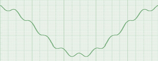
The data in the graph shown in figures 9 is a measured acceleration signal taken from a transducer mounted on an engine. If this signal is integrated without modification then the resultant velocity waveform looks like that in figure 10 with the large increasing ramp obviously caused by spurious DC or low frequency contributions.

If, however, the acceleration signal is high pass filtered at 5Hz then the resultant waveform still looks essentially the same as can be observed in figure 11. When the filtered signal is integrated, however, the resultant velocity waveform now looks like that in figure 12 and it clearly exhibits a more plausible form of oscillatory behavior.

Choice of high pass cut-off frequency

Commercially available analog vibration integrators typically choose high pass cut-off frequencies of 5Hz for Velocity and 10Hz for Acceleration. This is in the context of an expected analysis range of 10KHz, which means that as a proportion of the working range the filters are set to be less than or equal to 0.05% and 0.01% respectively. With Prosig’s DATS the user has much greater flexibility of choice of cut-off frequency, a fact that becomes increasingly important with signals that have low frequency bandwidths. If possible, it is preferable to choose a low-pass cut-off frequency that is no greater than 50% of the lowest frequency of interest; for example, when analyzing down to 6Hz the cut-off frequency should be set to 3Hz with a cut-off rate of at least 4 passes (8-poles). Normally, filters with Butterworth characteristics are used for both pre and post filtering, but others such as Tchebysheff can also be used although the user should be aware that the cut-off rates vary from filter to filter.

Pre and Post filtering

The concept of post filtering (after integration) was raised in the previous section. This is sometimes necessary to remove residual low frequencies / DC Offsets that sometimes appear after a signal has been integrated. (as in the engine vibration example illustrated above). The standard practice is to apply the same post filter as the pre filter.

Validation of Integration method

In order to verify that the combined filter+integration procedure gives the right result, it is useful to be able to validate the results using a deterministic input signal whose integral can be mathematically predicted. This can be easily carried out using the in-built signal generation facilities within DATS. For example, if one generates a sinusoid of amplitude 3.0, frequency of 10Hz with a sample rate of 1024 sample/sec, when this is integrated it should produce a cosine of amplitude . The corresponding value when calculated from the synthesized waveform using DATS gives an answer (after stabilization) of 0.04771 which represents an error of less than 0.1%.

The following two tabs change content below.

• Bio
• Latest Posts

Adrian Lincoln

Sound & Vibration Signal Processing Analyst at Prosig

Adrian Lincoln is an Applications Specialist at Prosig and works on signal processing applications, training and consultancy. He was formerly a Research Fellow at the Institute of Sound & Vibration Research (ISVR) at Southampton University. He is a Chartered Engineer and member of the British Computer Society and Institute of Mechanical Engineers.

Latest posts by Adrian Lincoln (see all)

• Averaging Frequency Response Functions From A Structure - June 17, 2016
• Seismic Qualification Testing (Part 1) - June 14, 2016
• What is Operating Deflection Shape (ODS) Analysis? - September 1, 2014