Amplitude And Energy Correction – A Brief Summary

Figure 4: Energy corrected spectrum

Amplitude And Energy Correction – A Brief Summary

Post author:John Mathey
Post published:September 1, 2009
Reading time:6 mins read
Post comments:13 Comments

Amplitude and energy correction has been and is a continuing point of confusion for many people calculating spectra from time domain signals using Fourier transform methods. The first thing to say, the information contained in data presented as amplitude and energy corrected spectra is equivalent. The only difference is the scaling of the numbers calculated.

Amplitude Corrected Spectrum

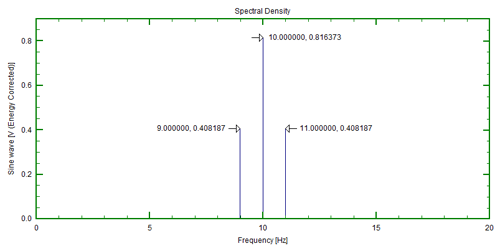
An Amplitude Corrected spectra is typically the default numbers you will find if you use a stand alone analyzer. Each frequency line of the spectrum is the RMS value of each frequency component of the time signal. If you have a 1Volt RMS sinusoid (as in Figure 1) and measure it with a FFT spectrum analyzer, the height of the line, or combination of lines that represent the signal will always add up to 1Volt RMS.

If the user does not apply any windowing to the time signal prior to calculating the FFT of the sinusoid and the frequency of the sinusoid is centered on the center of the FFT line of the spectrum, then the height of the single line will be 1 Volt RMS.

fig2 — Figure 2: Spectrum of 1 Volt RMS signal

Some confusion is added in when the user applies a time windowing function (typically a Hanning window) to the time signal prior to calculating the spectrum. Because the applied window narrows the time record (remember the time record is $1/\Delta f$ the frequency lines are broadened and overlap, consequently the single frequency sinusoid is now represented by 3 frequency lines (typically if the sinusoid is again centered on the center frequency of the specific frequency line of the calculated spectrum.

fig3 — Figure 3: Spectrum of 1 Volt RMS signal (with windowing)

This 1Volt RMS sinusoid hasn’t changed. Remembering, $RMS=\sqrt{Power}$ the sum of the power of the 3 lines of the spectrum must be equivalent to 1 V² (1 V_rms). It is obvious the center line of the calculated spectrum shows the 1 Volt RMS value so what are the other 2 lines at 0. 5 V RMS? The key here is the power associated with each of the spectral lines. To calculate the power represented by the spectra, one must square the values of each of the RMS lines

(0.5)² + (1)² + (0.5)² = 1.5 V²

But because we applied a Hanning window, the effective noise bandwidth for this spectrum is 1.5, we must divide the summation by this factor and then take the square root. The result is 1 Volt RMS as expected.

Remember, in general, calculating the Power of a spectra between frequency 1 ( $L_f$ ) and frequency 2 ( $U_f$ ) is the summation of the power in all frequency lines between frequency 1 and frequency 2 or:

$Power = \sum_{L_f}^{U_f}{Power_i}$

where

$Power = \sum_{L_f}^{U_f}{(RMS_i)^2}$

$RMS=\sqrt{\sum_{L_f}^{U_f}{(RMS_i)^2}}$

If the spectrum is amplitude corrected as described above, the summation of the powers (RMS²) is actually the summation of the powers in each line divided by the effective noise bandwidth of the measurement used or:

$Power = \frac{\sum_{L_f}^{U_f}{Power_i}}{1.5}$

$RMS = \sqrt{\frac{\sum_{L_f}^{U_f}{{(RMS_{amplitude})_i}^2}}{ENBW}}$

The effective noise bandwidth (ENBW) number is the product of the frequency line spacing ( $\Delta f$ ) and the effective bandwidth of the windowing function used (e.g. Hanning Window = 1.5). This effective noise bandwidth is included as a named element in all spectrum calculations performed with the DATS software.

Energy Corrected Spectrum

Amplitude and Energy correction of spectra is just a scaling factor. This scaling factor is the effective noise bandwidth of the analysis used, or in the case of a Hanning Windowing function, $ENBW = 1.5*\delta f$ .

If the spectrum is energy corrected for the same 1 Vrms sinusoid signal the scaling will look as follows:

fig4 — Figure 4: Energy corrected spectrum

Adding the powers in each line again requires squaring the RMS values, adding, then taking the square root.

$\sqrt{(0.408187)^2 + (0.816373)^2 + (0.408187)^2} = 1 V_{rms}$

As observed, the factor of the $\sqrt{ENBW}$ in the Amplitude corrected spectra calculations is already factored into the scaling of the Energy corrected spectrum, consequently, when calculating the rms level, one does not need to divide by the $\sqrt{ENBW}$ factor.

Now to calculate the overall levels between frequency 1 ( $L_f$ ) and frequency 2 ( $U_f$ ) one needs only to take the root sum squares of the RMS levels of each individual frequency line or:

$Power = \sum_{L_f}^{U_f}{Power_i} \,\,or\,\, RMS = \sqrt{\sum_{L_f}^{U_f}{(RMS_{energy})_i^2}}$

Converting Amplitude to Energy Correction Scaling

Equating the formulas for calculating the RMS gives:

$RMS = \sqrt{\sum{{(RMS_{energy})_i}^2}} = \sqrt{\frac{\sum{{(RMS_{amplitude})_i}^2}}{ENBW}}$

The special case encountered is when the frequency line spacing ( ${\Delta}f$ ) = 1 Hz making ENBW = 1.5 Hz. This means the difference between scaling of the amplitude and energy corrected spectrum is $\frac{1}{\sqrt{1.5}}$ or 0.816 .

Bio
Latest Posts

John Mathey

Senior Technical Specialist (Retired) at Prosig

John Mathey graduated with a MS degree from the University of Toledo in 1972. John gained over 35 years of experience with instrumentation, measurement, and analysis. Twenty-five of those years were spent at Ford Motor Company solving and providing training for vehicle noise, vibration, and harshness (NVH) issues. He was a technical specialist at Prosig USA, Inc. where he provided technical support to Prosig customers in the USA. Sadly, John passed away in 2022.

Latest posts by John Mathey (see all)

Exhaust Vibration Measurement – A Case Study - March 11, 2016
What Is Amplitude Quantization Error? - January 27, 2016
Creating An End of Line Vibration Test System - February 25, 2015

This Post Has 13 Comments

Yevgeni Tunik October 19, 2009 Reply
The text in the pictures is almost unreadable.
Emma Daly November 1, 2009 Reply
Hi, John
I am a final year engineering student and I am doing my thesis on damage detection using distributed accelerometer. In this I will be using the Fast fourier transforms and know very little about the topic. Is there any chance you have any information that will help me understand the basic? Any help at all would be greatly appreciated.
Emma
Chris Mason November 2, 2009 Reply
Hi Emma
I expect you’ve already had a look around the rest of the blog, but there are a couple of other posts that might help.
There is the article Notes On Fourier Analysis by Dr Mercer. This has some good illustrated examples and also looks at the mathematics behind the Fourier Transform.
Also, you may find 10 Great Fourier Transform Links helpful. This collects together several good WWW resources. One of the best links there is a series of lectures by Professor Brad Osgood of Stanford University. There are about 30 hour long lectures, but maybe the first few will help you.
Anyway, good luck with your thesis. If you have any specific questions then feel free to post a comment somewhere on the blog and one of our posters may be able to help.
Gareth Edwards April 14, 2010 Reply
John,
Good explanation for the ideal sinusoidal case. A couple of comments:
Equation 2 is incorrect – sqrt(1.5) = 1.2247…Vrms
It would be good to expand on this subject to include how to evaluate sinusoidal Vrms signals that are not located on a discrete spectral frequency. Or include the general version of Equation 6 which is the squared “area under the curve” as opposed to the sum of discrete spectral components
Eapen April 19, 2010 Reply
i have got some readings from a strain gage sensor,now should i remove the DC offset value to get the proper values or shoulldnt i…
John Mathey April 21, 2010 Reply
Thank you for your comment to the blog.
The answer to your question depends on what information you are looking for from the strain gage.
If you need know the static strain, then the strain gage sensor should be zeroed out prior to putting the component under load, then the DC offset value will be the component’s loaded static strain. The dynamic (vibratory) strain will be superimposed on the DC signal level. You might find the DC level will use up much of the dynamic range of the measuring instrumentation not permitting optimized gain settings for the dynamic signal.
If you are only looking for the dynamic strain due to vibration, then you can remove the DC offset value from the strain gage sensor signal. This will allow the channel gain setting to be increased to optimal levels for the dynamic signal.
I hope this response adequately addresses your question. Please feel free to contact me directly if you have additional questions.
John Mathey
PROSIG-USA
john.mathey@prosig.com
Matthieu Tessier February 25, 2011 Reply
Hello,
As part of a vibration measurement campaign, I’m being asked to provide acceleration levels. vibration spectrum and “complex of loads acting on a component (x,y,z)”.
The last item is not really clear to me.
I’ve previously heard of RSS values to obtain a single spectrum from a tri-axial vibration measurement.
How do I need to process my raw vibration data to obtain a RSS spectrum?
If anyone has an idea, please let me know.
Thanks and regards,
Matthieu
John Mathey May 6, 2011 Reply
Matthieu,
Calculating the RSS is simply a vector sum of the 3 orthogonal components s, y, & z.. In mathematical terminology it is x^2 + y^2 + z^2. Typically this is done on the RMS levels or amplitudes of the signals and not the raw time signals as the calculation includes squaring of the signals which will loose the phase relationship of the raw time signals. The RSS can be calculated using the Auto Power spectra or Power Spectral Density or any other RMS levels calculated (single numbers, order cuts, etc) for the x, y, and z signals giving a single spectrum.
The PROSIG software provides a module for performing this calculation on data curves (RMS vs time, RMS vs. frequency, etc….) . This module is call CALCRESULTANT and can be found in two places in the analysis menu or side panel under
Crash Biomechanics Calculate x,y,z Resultant
or
Human Biodynamics
Human Body Vibration Calculate x,y,z Resultant
This module also allows for individual weighting of the signals if one or more of the 3 directions are of more importance in your calculations.
I hope this feedback is helpful. If you have additional questions, please feel free to contact me.
John Mathey
Technical Support
PROSIG-USA
john.mathey@prosig.com
Jeremy December 16, 2013 Reply
Very good article, I often read that the correction for hanning window is sqrt(8/3), idenpendently of the frequency bin, quite different from the ENBW factor. And what is the effect of overlapping, like for the usual 50% overlap?
1. John Mathey December 16, 2013 Reply
  Jeremy,
  Thank you for taking the time to read this article. I am not quite sure where the sqrt(8/3) comes from. After all the numbers and formulas thrown out in the above article, the easiest way I have found to calculate the Energy corrected spectra is to calculate the spectral density (ASD or PSD) with units EU^2/Hz of the signal and then just take the square root of that spectrum. This gives the Energy Corrected Spectrum.
  As for your question on overlap processing. You might want to read the ariticle in our blog titled “Understanding Windowing and Overlapping Analysis”. You can find this article in the blog if you look for it in the index. The direct link to this article is “https://blog.prosig.com/2011/08/30/understanding-windowing-and-overlapping-analysis/”.
  I hope this information is helpful.
  John Mathey
  Technical Support
  PROSIG-USA
2. Seungha Lee October 12, 2017 Reply
  At first, thanks Mr.John Mathey for good article.
  As I know, sqrt(8/3) to be multiplied to values calculated from FFT with time data filtered by Hanning window compensate power loss of original time data by Hanning window. It’s exactly same as sqrt(power of original time data / filtered out time data through Hanning window).
Su July 4, 2018 Reply
Does this mean , if you calculate RMS values from PSD, do i need to divide by ACF and multiply by ECF.
Holman Araque May 25, 2020 Reply
Hi John,
I am trying to understand ENBW and all these topics. Could you please clarify how is affected the ENBW number when we have peak to peak wave amplitude curve instead of rms amplitude.