
The following article will attempt to explain the basic theory of the frequency response function (FRF). This basic theory will then be used to calculate the frequency response function between two points on a structure using an accelerometer to measure the response and a force gauge hammer to measure the excitation.
Fundamentally a FRF is a mathematical representation of the relationship between the input and the output of a system.
So for example the FRF between two points on a structure. It would be possible to attach an accelerometer at a particular point and excite the structure at another point with a force gauge instrumented hammer. Then by measuring the excitation force and the response acceleration the resulting FRF would describe as a function of frequency the relationship between those two points on the structure.
The basic formula for a frequency response function is

Where 
And 
And where 
Frequency response functions are most commonly used for single input and single output analysis, normally for the calculation of the 

Advertisement
Some examples of the products from the CMTG brands
DJB Accelerometers
Sense

- Piezoelectric charge & IEPE accelerometers
- Instrumentation, cables & accessories
- Calibration & repair service

Prosig DATS Hardware
Capture

- Rugged, mobile data capture
- Options inc. 24-bits @ 300k samples/sec
- From 4 to 1000’s channels

Prosig DATS Software
Analyze

- Don’t just test – gain insight from your data
- Huge selection of signal processing algorithms
- Optional application add-ons
The
The
Additionally, there are other possibilities, but they are outside of the scope of this article.
The breakdown of

Where
And 

And where 
In very basic terms the FRF can be described as

The breakdown of

Where
And 

And where 
In very basic terms the FRF can be described as

In the following example we will discuss and show the calculation of the
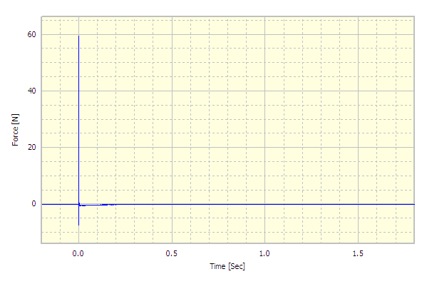
The excitation or input would be the force gauge instrumented hammer, as shown in Figure 1 as a time history.
In this case the response or output would be the accelerometer, as shown in Figure 2.

However, as discussed earlier, the frequency response function is a frequency domain analysis. Therefore the input and the output to the system must also be frequency spectra. So the force and acceleration must be first converted into spectra.
The first part of the analysis requires the Cross Spectral Density of the input and output, this is 

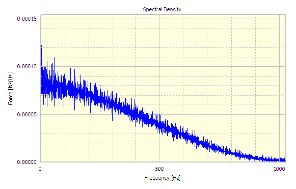
Next, the Auto Spectral Density of the input or excitation signal is required. This is calculated using the Auto Spectral Density Analysis in DATS, this analysis is sometimes known as Auto Power, the result of which is shown in Figure 4, this is
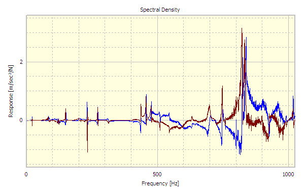
The Cross Spectrum is then divided by the Auto Spectrum and the resulting frequency response function is shown in Figure 5.
The response function would normally be shown in modulus & phase form as shown in Figure 6.

The entire analysis as used in the Prosig DATS software is shown in Figure 7. The data flow from the original input and output, force and response, can be seen through to the frequency response function. The DATS software does, of course, provide a single-step transfer function analysis. We have deliberately used the long-hand form below to illustrate the steps in this article.

It is necessary to understand that for the purposes of understanding and clarity in this article some important steps have been glossed over, windowing of the input for example, to allow the basic understanding of what makes up the frequency response function.
James Wren
Latest posts by James Wren (see all)
- What Are dB, Noise Floor & Dynamic Range? - January 12, 2024
- How Do I Upsample and Downsample My Data? - January 27, 2017
- What Are Vibration, Torsional Vibration & Shaft Twist? - November 8, 2016

Hello,
Normally people don’t expect to see an Autospectrum, or Power Spectral Density on a linear scale, and it looks so noisy, that I suspect the impact was recorded using a Hanning weighting – a common mistake.
The end result, – the transfer function is also odd, to my eyes.
I would have expected a bode plot.
I am aware that linear display is useful for fatigue and stress purposes, but the frequency range is too high for this to be the application.
Hello to get Natural frequency of any structure , if we are using modal Impact hammer and Accelerometer then FFT of Accelerometer signal
(as a response to impact of hammer)represents Natural frquency?
Hello Samruddhi,
Thank you for asking a question on our blog.
To find the natural frequency of a structure you would complete a hammer impact test with a force instrumented impact hammer and an accelerometer, sometimes called bump testing or tap testing.
Taking the FFT of the response signal, converting the result to modulus and phase and taking the real part only will not give you a complete picture of the part under test. Also you’ll be missing out on important issues like excitation and response windowing, so potentially the results could be corrupted.
The transfer function method is more reliable and will give higher quality results, hence it’s use in industry.
Dear Wren,
My question is related to the FRF (magnitude) vs frequency plot. I recently worked on the modal analysis of woven composites. Some of the FRF vs frequency plots don’t have very sharp peaks. The peaks are a little skewed for some of the plots. I was just wondering if I apply half power bandwidth on these plots, would it be validated?
Faithfully,
Khizar
Hi Ken,
Thanks for posting on our blog.
I’d like to respond to your points if I may.
I understand your point of view, the Power Spectral Density is normally shown on a logarithmic scale (Y axis) as you suggest.
However for the purposes of this article it is not, we have shown it as linear. Here in this article we are trying to explain and discuss the basics in a straight forward simple fashion.
With regards to your points about noise and windowing, we apply a window to the force signal. We also apply a window to the response if it is very noisy, but we prefer not to do this.
The window is an exponential window, like a transient window for example. It is not a hanning window or similar.
The structure in question is a very simple structure, if a little noisy, and you’re correct it’s not being used for fatigue analysis.
With regards to the final output, our DATS software can quickly switch between Modulus & Phase and Real & Imaginary. So it is possible show in the Bode format you mention.
what can be infered from figure 5,please explain..
Hello Eapen,
I’m not sure anything can be inferred from Figure 5, it simply shows the Frequency Response Function for this particular test.
how can v obtain auto spectral density of velocity from auto spectral density of the displacement
Hi Kiran,
Thanks for asking a question on our blog.
This conversion is one of the fundamental laws of Newton’s physics.
It is possible to convert from Acceleration to Velocity to Displacement using calculus, specifically integration.
Our Prosig software performs this conversion in an advanced fashion to take account of the constant and remove this error from the results.
You should keep in mind that the original time series is required for this conversion.
If you would like to discuss this feature further please feel free to contact us directly.
Hi
Just say you have several accelerometers on a complex vibrating structure. Each accelerometer has a slightly different frequency spectrum. Lets also pretend that you have a mic at some distance from this vibrating structure, and that you are trying to locate the particular component or part of the structure that is responsible for a radiating a particular tonal frequency. Would the cross spectrum be valuable in identifying which accelerometer is the culprit of this offending sound?
Many thanks
Hello Paul,
Thanks for asking a question on our blog.
We can see that you have a good understanding of what you are trying to do.
In our opinion the Cross Spectrum is a step in the correct direction, but you should go one step further and calculate the Coherence between each vibration source and the microphone response, you can do this very easily with a software package like DATS.
To actually rank each vibration with respect to the microphone you should consider something like the Source Contribution Package, again as part of DATS.
The Source Contribution Analysis uses a method called Singular Value Decomposition. The Singular Value Decomposition computation produces an eigenvector matrix, this matrix is used to derive the cross spectra between the vibration references and the measured sound response. These cross spectra are then used to calculate the Reference Related Auto spectra at the response position. Each Reference Related Auto spectrum is related to the coherent contributions from the particular references and source input.
If you would like to discuss this further please feel free to contact us directly.
Going back to Paul’s hypothetical situation. Suppose that the accellerometers are measuring the start of an event that will be producing the noise that is being measured, but that there is no real reason to expect there to be any frequency correlation between them, would any conventional analysis work then?
For example, if you have 5 drums and a lightbeam sensor for each drum that triggered just before the drumstick hit each one, and that the drums are being hit in a regular sequence. How might one analyse the data (one mic channel and 5 drumstick sensors) to determine which drum was loudest/highest-pitch etc?
Hi Andy,
Thanks for asking a question on our blog.
I think there is some difference between your question and Pauls.
In Paul’s case the vibration responses are all related.
In your case they are not.
Therefore the same analysis would not apply.
I think you are trying to find which drum gives a certain frequency response when hit. The easiest thing to do would be to use a microphone, mounted about the drums and hit each drum in sequence. Starting and stopping a data capture for each drum. Then simply frequency analyse each of these data captures. You might need to do it several times to build up an average for each drum as you may hit it differently each time.
This will give you the full frequency spectrum for each drum.
You wouldn’t need any accelerometers at all.
Sorry, perhaps I took my analagous situation too far. This is actually exactly the same question as Paul’s, but we have a slightly different conception of the nature of the data. I should perhaps have chosen a better analogy, as the trigger pulses occur at 20-150Hz which would be a pretty inhuman rate of drumstick operation.
Hi Andy,
Thanks for the additional information, but I still don’t understand your application and can’t comment on it unless you can explain what your trying to do. Perhaps you could contact us directly to discuss?
I am looking for the information about the engine order, used for frequency response analysis.
We are working on frequency response Analysis for the exhaust systems, there we use different engine orders, i.e. 1st, 1.5, 2nd, 2.5 etc orders. Kindly let me know what is the actual meaning of this engine order. All I know is, its the disturbances created per rotation of the crank shaft. I need information.
– Ashujc 🙂
Hello Ashujc,
Thanks for asking a question on our blog.
An engine order is really two separate words, ‘engine’ and ‘order’
Engine is obvious but ‘order’ not so.
You could have an order of anything that rotates, not just an engine. For example wind mill blades have their own orders.
An order is the speed that something happens at.
So if a shaft is rotating at 100 times per second you would have a fundamental frequency of 100Hz. If there were two blades on opposite sides of the shaft somewhere long it’s length, this shaft they would be causing an excitation or noise at 200Hz because there is two of them. You could say the noise from the blades is a 2nd order noise of the main shaft.
The same goes for any other number. An order is the relationship to the main fundamental frequency that occurs in multiples of the fundamental.
Can I use the peak value of a frf curve as resonance frequency or I should convert it using any mathematical equation? If yes then which equation should be used?
Hello Sania,
Thank you for posting a reply on our blog.
The first mode or resonant frequency is the frequency at which the FRF shows a corresponding 180 phase shift.
In a simple structure like a tuning fork the frequency of the resonance will be the highest amplitude in the FRF. But it more complex structures this is not always the case, infact often it is not the case.
So the answer to your quest is No, you cannot use the peak value in the FRF as the frequency of the resonance.
I believe the article https://blog.prosig.com/2012/08/20/what-is-resonance-part-2/ will provide further information.
It might be worth reading the complete resonances articles at,
https://blog.prosig.com/2007/05/23/what-is-resonance/
https://blog.prosig.com/2012/08/20/what-is-resonance-part-2/
https://blog.prosig.com/2013/07/17/what-is-resonance-part-3/
James,
Thanks for a clear example.
Would be more useful if you could publish the parameters used by DATS.
e.g.
Sampling rate:
Anti-aliasing filter:
Number data in each FFT:
Windowing:
Ya
Hello Ya Huang,
Thank you for your feedback.
We wanted to keep the article as simple as possible, so we have kept away from any specific numbers and data, just the main principles.
If you would like to discuss in further detail, please feel free to contact us directly.
Hi James,
Your example is very instructive. However as a new comer in FRF, I could not figure out how you obtain the phase for FRF from the steps mentioned in figure 6. Obviously the division can only give a real number, which is the amplitude of FRF. Thanks.
Hello Steve,
Thank you for asking a question on our blog.
You have closely studied figure-6, which is good to read.
In figure-6 the CSD (Cross Spectral Density) is divided by the ASD (Auto Spectral Density). The CSD is a complex number, the ASD in a real number.
Any mathematics that involve a complex number will result in a complex answer, so the answer will have both a real and imaginary part or expressed differently a modulus and phase.
For example.
Where the CSD is represented by A+ iB, where A is the real part and iB the imaginary part.
And where the ASD is represented by C, where C is real.
The formula in figure-6 would be,
(A+iB) / C
Which is exactly equal to
A/C + i(B/C)
If you have any further questions, please feel free to ask.
I’m reading this because I’ve just been sent a newsletter that points to the page.
Are you sure you should really be advising use of H1 and H2 on single tap test recordings?
You see I agree with your first equation H(f)=Y(f)/X(f) but the subsequent equations are unhelpful if you end up using segment averaging (inherent in the calculation of the power and cross spectral densities) on a single tap. The windowed data for the force time history segments will all be zero except for the one window that contains the actual impact. Moreover the response in the subequent windows has nothing to do with the corresponding force window leading to potentially significant bias errors in the transfer function.
If you must use segment averaging to obtain transfer functions for tap test data then I think you need to make it very clear that this is for multiple taps and that the window length used must exactly correspond to each tap and response time history (i.e. there must be no segmentation within each time history pair) and the window length must be sufficient to capture the full decay of the vibration following the tap. Your readers should also know that the highlighted inappropriateness of segment avergaing for tap test data cannot be overcome by multiple taps at random intervals – that only compounds the errors introducing rippling in the estimated transfer functions because of the [Fourier transform properties of the] inherent similarity between one tap and the next.
Hello Stuart,
Thank you once again for your comments.
First of all I can only comment on the software we produce at Prosig and the methods we would recommend.
This article is intended to give a basic understanding of the concept of what we call Hammer Impact tests or you refer to as Tap tests.
For Hammer Impact Analysis we do not use or suggest overlapping segments, we would indeed suggest this is an incorrect method.
So I agree with your points, it is just you have assumed we use a method we do not use or recommend.
Our Hammer Impact software uses a Wizard to set-up the sample rates and durations to match exactly. The data is then processed as one entire block, including a pre-trigger. A force block and response block, having had force and response windows applied.
Thanks again for your comments.
Hi,
I have done FFT analysis on mild steel beam of 1 meter length and I was looking frequecy of mild steel on first three modes. After performing the test I have got auto spectrum input response graph and frequency response(response,force)input (magnitude) working graph. which graph is best to consider for the frequency?
Umar.
Hello Umar,
Thank you for asking a question on our blog.
You question is quite straight forward.
You should have a frequency response curve from each of your accelerometers, these should give you a basic idea of how the structure is behaving.
If you want to understand further then I would recommend the output over input method as detailed in the article.
If you have further questions, please ask.
Hi,
Thanx for the reply, I just want to ask that what is the difference between Autospectrum response graph and Frequency response graph because they are giving same results.. and how can i find the length/breadth ratio against frequency plot, of a rectangular beam with the length= 1m and breadth= 0.039m.
Umar.
Hello Again Umar,
You might be asking questions that are too specific for us to do able to answer directly without more details of your project.
With regards to your question on the difference between an Auto-spectrum Response and a Frequency Response Function, I’ll try to explain step by step.
The Frequency Response Function is a measurement of motion per unit area. It is a Complex quantity and importantly has phase. The main point for the FRF is that it is related to the input force that is exciting the structure.
The Auto-spectrum Response is a measurement of the motion only, there is no phase component. Additionally the Auto-spectrum Response is not related to the input force that is exciting the structure, but only to the response of the structure.
Hi,
Is there any way to estimate frf only from output data. Say, I have accelerometer output for vibration of a bridge under traffic etc over a period of time. Can I generate frf without knowing force.
Thanks a million,
Krishna
Hello Krishna,
Thank you for asking a question on our blog.
A frequency response function is a measure of an output of a system in response to a given input.
So in short no, you can not use only responses to create an FRF as detailed above. You can however calculate the Transmissibility between several accelerometers if you define one of them as a reference.
But it depends on your objectives and w hat your trying to achieve.
Hi James,
Let’s say I plan to perform a modal test on a quite complex test article. For this test, I will have 20 accelerometers scattering around the test article. Now, if I selected one location to hit with an instrumented hammer to excite the modes. Based on your explanation about the FRF, in this example, I would have 20 FRFs generated by DAT (each FRF represents the response relationship between the impact point with respect to one of 20 response points where the accelerometers are located). Now, my question is: “Can the resonance frequencies of the test article be identified by examining the modulus & phase plots of the FRFs?”. If yes, then how to identify those resonance frequencies?. Thanks.
Hi Nikk,
Thank you for asking a question on our blog, it is always good to talk to people who are performing tests, ‘at the coal face’ we say.
Yes your correct, if your using uni-axis accelerometers and you do as described you will have 20 frequency response functions. I would suggest that the impact point be near or on one of the accelerometers, but you do not have to do this.
Yes, your right from the Modulus and Phase plots of the FRF’s you will be able to identify the frequencies of the resonances.
As a rough rule a resonance will show itself as a peak in the Modulus plot and as a flip of the angle in the Phase plot.
James,
Thanks for the response. I have 2 more questions for you:
1) You said: “as a rough rule, a resonance will show itself as a peak in the Modulus plot and as a flip of the angle in the Phase plot”. According to this sentence and after looking at the sample Modulus/Phase Angle plots in Figure 6 posted on your blog above, the Modulus plot has many peaks and the Phase Angle plot has many flipped points (0 to 180 degrees), so how do I know which peak in the Modulus plot associated with a flip of the what angle in the Phase plot is a correct resonant frequency?
2) Looking at Figures 3 and 5 posted on your blog above, there were 2 different colored curves (red and blue), and I wonder what did red and blue curve represent?
Hello again Nikk,
I’ll address your questions one by one,
1,
There is no right or wrong answer, life is never that simple. But the resonance will normally be shown by the largest peak in amplitude. Find that peak and then check the phase if the phase has inverted at this point then you have probably found the resonant frequency.
Often your better off to view the data in a log form, like that shown here.
Then you can clearly see a resonance and the corresponding change in phase.
Do be aware there is no magic or easy way to do this, you have to understand the structure your testing and have some ideas yourself before you even do any testing, testing should validate your ideas not the other way round.
2,
Figures 5 & 6 show the same data.
Figure 5 shows the data in complex form, sometimes known as real and imaginary form. By default in our DATS software the real part is shown as blue and the imaginary part is shown in red.
Figure 6 shows the same data in modulus and phase form.
The signals are exactly the same just shown in different ways.
As an engineer you should consider the modulus and phase form.
Hi James:
This is great! I actually need to calculate the FRF for an experiment. I have the excitation acceleration signal and an acceleration response singnal in time domain. I am new to signal processing and would like to know in detail about the meaning and numerical computation of auto and cross spectrum in order to compute the FRF. I hope you could guide me to something useful for understanding the underlying concepts. Any insights into computing the FRF for my case would be great!
Thanks.
Rummy
Hello Rummy,
Thank you for asking a question on our blog.
To compute the FRF (Frequency Response Function) in your case is quite simple,
Step 1
You convert your time series signals to the frequency domain using an FFT algorithm
Step 2
You divide the response signal by the excitation signal
You then have your resultant FRF
You mention Auto Spectra and Cross Spectra, you could use the following method,
Step 1
Calculate the Cross Spectra of the Excitation and Response
Step 2
Calculate the Auto Spectra of the Excitation
Step 3
Divide the Cross Spectra by the Auto Spectra
You then have your resultant FRF
In our Prosig DATS software we have a simple function that takes a time series or a frequency spectra excitation and response and produces the FRF for you.
hey thanks James. I think I have some good initial idea now to build upon. Cheers!
I am new to signal processing and french speaking; so I hope that these two drawbacks will not make my questions become too stupid.
My problem is about structures on which à kind of wind tunnel test has been made. In the case were a single excitation point is used, say A, then at each frequency w, a transfer function from the input towards an output quantity B exists, Hab(w) .
Then the power spectral density of the ouput quantity B is said to be Sb(w)=|Hab(w)|².Sa(w)
(Sa being the power spectral density of the input quantity A)
Now what if the input is divided in four points ?
If Saiaj(w) is a cross spectral density of
input j versus input i, can I consider |Sa1a1(w) Sa2a1(w) |
an input cross spestral matrix, being that : [SIN]=|Sa1a2(w) Sa2a2(w) |
and then how can I use it | a4a4 |
to obtain the output responses ? And How ?
Thank’s a lot to explain me these basic things,
David
Hi David,
First of all can I ask if you are measuring forces or just responses? Also do you know if the input signals(forces) are independent from one another? (If they are independent then the coherence spectrum between any pair of signals will be approximately zero.) If the input forces are indeed independent then the output will be a simple summation of the responses to the individual inputs. However, if the inputs are not completely independent then the predicted response is not so easy to calculate as it requires the computation of the partial coherences between the inputs. If you can tell me a little more about your test situation then I can give you more appropriate advice.
Adrian
Hi Adrian,
thank’s a lot for having spent some time with my question. As an answer to your first question, please take in account that I am stress analyst, thus the data I’m interested in is neither forces nor displacement responses, but stresses. But our stress analysis software knows how to convert displacement responses towards stresses.
Secondly, the sources acting on my structure are not completely independent; they are aerodynamic noises on different parts of a same structure. It is an aircraft component which size is slightly smaller than a meter, and six micros have been fixed on it during the wind tunnel tests, in order to measure the input PSD’s.
If I call Sa(w) the input PSD (in Pa²/Hz since it is that of an acoustic pressure),
and Sj(w) the output PSD, (in MPa²/Hz since it is that of a mechanical stress),
and Hja(w) the transfer function from the pressure towards the stress at rotating frequency w :
Then for each w, Sj(w)=|Hja(w)|².Sa(w)
And I am interested in the RMS value of that stress over a certain frequency band of the aerodynamic noise.
Now let’s see what happens when there are, say just two input zones, a and b.
There is an input direct PSD over zone a, say Saa(w),
there is another input direct PSD over zone b, say Sbb(w),
there are two input cross PSD’s, say Sab(w) and Sba(w) which should be its complex conjugate. (Tell me please if it is true)
Then for each w, the output PSD is Sout(w)= ?j=a,b ?i=a,b ( hi(w).hj(w)*.Sij(w) )
And I am still interested in the RMS value of that stress over a certain frequency band of the aerodynamic noise.
Now let’s see what happens when there is only one input zone, but two distinct PSD’s acting on it. For simplicity I input within the stress analysis program that I use, that the cross PSD’s are almost zero, say 1.E-12 or 1.E-18 times the product of the two input direct PSD’s.
That is the point that I want to know; is it possible to “add” two PSD’s acting on the same area, with almost zero cross PSD’s.
It seems to me that I could.
I am very glad to be able to write such a text as above, as I feel a bit more “clever” about signal processing. Please continue telling me if what I wrote above is plenty of sense or not, and feel free to ask anything if you feel that some questions or answers may make me progress in that domain.
Thank’s again,
David
My structure (steel) in question is small, thin and light. I cannot physically attach any accelerometers, as the mass and cable tensions would alter the frequency response. So I use non-contact displacement measurements (like Laser or Capacitance Probe or EC probe). Also – I cannot use the typical impact hammer as well – I might brake the structure. I can may be drop a small steel ball on the structure to provide excitation.
Two questions.
1. Since direct excitation measurement (impact hammer) is not possible, can I measure the impact force by dropping the same ball on top of the accelerometer or load cell on a separate run?
2. If Q1 is possible, then I’d have input data in accelleration, and output data in displacement. What should I do from here?
Thank you very much for your time.
Hi Jay,
Thanks for asking a question on our blog, it sounds like you have an interesting application.
We understand the restraints your working too, things in life are never simple and never have easy to follow guidelines.
1,
Yes, you could drop the steel ball on to the accelerometer, but I thought you said you could not attach an accelerometer to the structure? I would have thought if you could attach an accelerometer and drop a ball on it, you could use a very small and light force hammer. But the accelerometer method is fine if that is all you can do, maybe there is some practical restrictions that mean you can’t perform the test exactly how you would like to.
2,
There is no issue with the type of data, however acceleration as an input and displacement as an output would be a Transmissibility function, not a transfer function, transfer functions should have force in some way. In short, it is not really an issue.
Please feel free to pose further questions if you desire.
James thank you for reply.
Sorry for the confusion. What I meant by “dropping a ball on the accelerometer” was, to setup an accelerometer on a flat table (not on the thin structure in question), and drop a ball on it to see how much impact the “ball dropping” can deliver.
Originally, I was thinking of shooting the ball using a BB air gun to deliver the impact. If I shoot the ball on an accelerometer (provided distance and airpressure would be consistent), I would know how much impact there is, and assume that the same amount of impact will occur when I shoot it to my thin structure in question.
I hope this makes sense.
Hi Jay,
Thank you for coming back to us and asking another question.
I understand, thank you for the clarification.
In short no, you can not do that.
You have to measure the excitation into the structure, not the input into another structure.
For example if you put the accelerometer on a solid rock and dropped the ball bearing on it, then put the same accelerometer on a fluffy pillow and dropped the same ball over the same distance on the accelerometer, you would not see the same duration or magnitude response on the accelerometer. In short the input into the structure would be different.
I would suggest the best solution for you might be OMA or Operational Modal Analysis. Often when people are discussing hammer impact testing they incorrectly refer to hammer impact tests as modal analysis, it is not.
In any case you could place the structure on a shaker table and then use that shaker control signal as your input, then use the selected sensor to measure the displacement as a number of points on the structure.
Please let us know if you have further questions at all.
Hi James:
I have a question related to FRF computation for transient input-output signals. Would it be OK to compute the FRF of a system by only considering a certain transient region, instead of the entire time-history (i.e, before the signals die out) ?
Thanks and regards
Hi Rummy,
Thanks for asking another question on our blog.
The short answer is No it would not be OK to only consider the transient region.
The long answer is that you should not do this because the definition of a transfer function is that your measuring the input and output to a mechanical system. There will be a phase delay in that system. Thus if you end the time series too early, you may miss part or all of the response, and thus the frequency response function would be based on partial and incomplete data.
This is not the only reason that you should analyse the entire time series, but it is the main reason.
From a signal processing point of view the time series signals should be zero at the start and zero at the end. If they are not you will get noise at every frequency of the frequency response function. To get around this windowing is often used to attenuate the responses down to zero by the end of the time series if they are not there already.
I hope this helps and is clear.
Hi James,
I,m new to signal processing. I would like to know how you calculate the dynamic stiffness,Kd from this curve. How would you calculate the Kd at any random point on this curve other than peak responses.
Suppose I’m plotting an FRF graph taking magnitude(0-120db) on Y-axis and frequency(0-600Hz) on X-axis. I would like to calculate dynamic stiffness,Kd using this graph using least square method, rms method, average method.
Also how it differs if it is undamped,underdamped,critical damped,overdamped structure. How to change the spring/bush stiffness values using damping values.
It will be of much help if you can explain this in a simple way with the formula used for calculating the above.
Thanks and regards
Hi James,
I have forget to say that I’m interested in acceleration as output response and accelerance(acceleration/force) as the magnitude on the Y-axis.
Hello Prasad,
Thank you asking some questions on our blog.
You certainly are asking a lot on quite a broad subject. I think your requests might well be outside the scope of the original article which doesn’t cover dynamic stiffness or indeed stiffness at all.
I’m not sure you would calculate a dynamic stiffness curve from a transfer function like that detailed in the article. Indeed the dynamic stiffness would itself be a transfer function.
I think for dynamic stiffness you have to consider a few basic principles. The input into a system is going to be a F (Force) and the output R (Motion) which is measured as a displacement. The dynamic stiffness of the system is the relationship, or transfer function between the two parameters listed above.
I would suggest that it may be best to research further in the field of structural dynamics for further information.
Please feel free to post back what you find.
Thank you James for answering my question earlier today , I hope I am not taking lots of your time .
First of all I would like to congratulate your company to have an outstanding intelligent person like yourself . From the nature of your answer I can see that given the fact I am student at Aberdeen university ,
You will note that some of the facts I studied in the past I only understood it from theoretical point of view with no physical understanding , I am finding your comments are EXTREMELY useful .
It would be greatly appreciated if you could possibly make useful comment or answering the questions in simple way .
In the embedded figure you attached Nik , I can see that there are three peaks , two of them are for the Zeros of the systems and one of them for the Pole where is the resonant peak occur .In your answer to the question I found in determining the peak ,, the phase will be inverted .
Question 1) To what extend the phase shift is required for peak resonant is occurred , is it necessarily to -180 or depend on the order of the system , for example the phase inverted by -90 ? Also would the sign make difference if it is +180 or +90.
Question 2) Looking at the zero peaks in my system they are below 0 decibel different than the one on the figure . Do you have any physical comment about those peaks occurring in the frequency response for the zeros ? I can also see phase shift inversion at those peak ?
Question 3 ) In my system The Bode diagram shows a 180° phase lag at every resonant frequency and a 180° phase lead at every anti-resonant frequency. This is a characteristic of collocated systems.? I do not understand this clearly as you have excellent skills in showing the material in more physical understanding .
Question four )
The in-bandwidth zeros of the system are highly dependent on the out-of-bandwidth poles ? what does that mean if you have more clarity it would be greatly appreciated
question five )
if I want modify system from containing resonant poles followed by interlaced zeros, to zeros followed by interlaced poles ? in terms of stability what does that mean , can you please clarify things for me clearly.
Hello Mohammed,
Thank you for posting some questions on our blog.
We will try to answer your questions as best we can.
1,
The sign doesn’t make a difference and it doesn’t matter where you start, the inversion will be just that, 180 degrees.
2,
There are resonances and anti-resonances, it sounds like you have found some anti-resonances.
3,
I’m not sure I understand your question, it seems more like a statement. Your using a Bode plot and have noted a phase change along with amplitude peaks. You would appear to have found resonances.
For your final questions I would refer you to a sister article,
https://blog.prosig.com/2014/04/10/how-do-we-design-or-modify-a-system-to-avoid-resonance/
This should give you some basic design pointers.
Hello James,
I am new to practical testing & signal processing.
I have few question about selecting excitation and response points.
1) How do we select excitation and response points for practical component FRF testing? I mean if I hit structure with hammer in X direction do I need to take response only in X direction or response in Y,Z directions as well? or Do I need to hit separately in each direction (Y,Z) and take response in (Y & Z respectively)?
2) Do I need to select input point near mounting point of component while doing component FRF or at free end of component?
3) Different response points give different amplitude values but peak frequency could be same (Correct me if I am wrong). How do we make sure which response point gives us proper frequency and amplitude values?
What is your suggestion?
Thank you,
Dhruvit
Hello Dhruvit,
Thank you for posting on our blog.
We would be happy to assist you as much as we can.
Question 1,
There is no right or wrong answer.
Generally one would excite in an axis, perhaps the X axis and measure the response in one or three axis.
However to be ‘more’ correct one should measure the response in the three axis and excite three times, once in each axis, thus you would have 9 FRF’s.
These can then be analysed individually or averaged as per the users requirements.
It really depends on the structure your testing, take a point on a bell for example, hitting the rim of the bell in the X or Y axis would make little difference, but hitting in Z axis could/would produce difference excitations.
So it depends on the structure or components your working
Question 2,
Personally I would test the entire structure in the free free state (suspended in free air) first of all and then in it’s restrained state, that is mounted.
Looking at the differences between these usually provides some interesting discussions.
Question 3,
Amplitude is not relevant in this case, actually the FRF’s will be unit less so there is no concept of amplitude. I refer to the bell or tuning fork example, the amplitude will be different but the frequency will be the same at any mounting point within reason.
As to the question how do you select a position to give you what you need, you test in all locations to understand the component, once you understand the component you can select the best positions for future testing.
Please feel free to ask if you have more questions.
Dear Mr.James
I have a question…i have tried harmonic analysis of the Cantilever beam in ANSYS. i got FRF but i need to find the mode shapes through FRF so that i am able to compare the experimental results….cab you help me in any way…
i also have another question, can you throw light on the real and imaginary part of an FRF
Hello Sudeep,
Thank you for posting a question on our blog.
Your asking two questions,
1,
How do you find mode shapes.
2,
Please explain the complex numbers used to store and display an FRF.
Here are your answers,
1,
Usually you would perform a hammer impact test or a tap test, to find the FRF’s of a structure. Then you would animate the data as a wire frame model or mesh.
The animation of this mesh will allow the user to visualise and find the frequencies of Mode 1, Mode 2 and so on,
To do this with Prosig equipment, a P8000 device is required, with the Prosig Hammer Impact testing software and the Prosig Structural Animation software suite.
Further, you could use the Prosig Modal analysis software on the FRF’s directly from the Hammer software or another source, and find the modal frequencies and damping factors directly.
2,
Generally speaking FRF’s should be stored as complex numbers, however the human brain really doesn’t understand complex and works in a modulus and phase way.
Hence a complex FRF is usually shown as Mod Phase display, even though it is complex when stored.
Dear Mr.James & Mr.Sudeep,
I have the same simulate in Ansys for the harmonic analysis of the Cantilever beam.
All data based on this article “A frequency response function-based structural
damage identification method, Usik Lee *, Jinho Shin” (I can not paste the chart at this comment). But I can not have the peak of FRF the same with my reference.
So can you share with me some reference about how to create FRFs chart on Ansys? I am a PhD student at the Vietnam university. It is a pleasure for me if you reply me on my email: “nguyenhoangquan72@gmail.com”.
Thanks & Best Regards,
Quan
Hi Mr. Wren,
I noticed that in the impact signal there is a negative part to the amplitude right after impact, resulting from some kind of recoil in the hammer load cell (I guess). Is it normal to get this considering this is a negative force? I am getting similar results but the negative amplitude is almost equal to the positive part. Can you please elaborate on this and how to take care of this in FRF calculation.
Thanks,
Salman
Hi Salman,
Thank you for posting a question on our blog.
I understand your point and I have seen the behaviour your observing several times before.
First of all, yes, any structure will behaviour a little like a spring, so when you make the impact with the force gauge instrumented hammer it will bounce a little, this bounce or ring will be caused by potentially several factors, but will result in a negative spike or number thereof after a positive spike.
It should be small however and should not adversely effect the results.
This however is not what your seeing, from what you have described a negative spike that has a magnitude the same as the positive part could well mean there is another issue.
I have seen this before when the force instrumented hammer is not an isolated sensor and the structure being impacted is either not (well) grounded or has another ground to that of the sensor and front end. In short when the hammer is impacted the gauge electronics actually gets moved to another zero volts and hence the reading’s are knocked off. Sometimes I have seen a negative going only pulse as the electronics int he hammer are overloaded.
It depends if your using a metal tip on the hammer or not, if you are using a conductive tip try using a rubber tip or none conductive tip, thus there is no electrical connection between the hammer and test structure.
The best solution would be check and improve the ground for the test structure and the front end/sensor.
You should get a positive going pulse similar to that in the article in most if not all cases.
Hello James,
Great article and blog. I just have a few questions:
1. You mentioned that you windowed the input signal, but not the output. Under what circumstances would you also window the output?
2. Are there any differences to calculating the FRF using the ratio of FFT’s vs. CSD/ASD? Which do you prefer and why?
3. I’m a little confused about using the FRF (e.g., accel/force) vs. the transmissibility (accel/accel) to calculate structural properties such as damping, etc. In other words, if I do an impact test and get an FRF in units of (m/s^2)/N, then do a base excitation on the same structure to get a dimensionless transfer function (dB or gain), will the half-power method give me the same result for the damping ratio for both tests? If this is outside the scope of this article, could you point me to a reference that might answer this? Thanks!
Hello Lee,
Thank you for asking some questions on our blog.
I will try to answer your questions as best I can.
1,
In simple terms I would window in any situation where the structure being testing is still ringing at the end of the data capture window.
The objective with windowing is to reduce the ‘ringing’ to zero by the end of the capture window. So the signal starts and ends at zero in all cases.
So imagine a tuning fork, you impact it and it starts to ring. Your capturing data for a finite amount of time, the software will have selected a time to capture based on your requested frequency range and frequency resolution (FFT block size), is the test structure still ringing? If so you need response windowing. The same applies to the excitation signal.
Our software walks the user through a dummy test and if the structure is still ringing then a response window is applied automatically for the user as required, again the same applies for the excitation.
Generally you would apply the window to the output or response signal and very rarely the input or excitation signal.
2,
There are differences for sure, that is why there are different ways of making the calculations.
The most common types are H1 and H2, but there are many, many others.
For example Prosig DATS supports;
H1, H2, H3, H4, Hs, Hv, Hc, Hr and H0.
You will probably be aware of H1 and H2, (there is no need to go into the others here)
H1(f) = Gxy(f)/Gxx(f)
H2(f) = Gyy(f)/Gyx(f)
Where Gxy(f) is the cross spectral density between the response signal y and the reference signal x, Gyx(f) is the complex conjugate of Gxy(f), Gxx(f) is the auto spectral density of the reference signal and Gyy(f) is the auto spectral density of the response signal.
In almost all cases people will know of or use H1 or H2,
H1 is the classical estimator and is used in situations where the output of the system is expected to be noisy when compared to the input.
H2 is the inverse of H1 and is used in situations where the input of the system is expected to be noisy when compared to the output.
But when it comes to my personal preference, I like to keep it simple and when dealing with transient signals I would use,
H(f) = Y(f)/X(f)
Where the resultant transfer function is H(f) and where Y(f) is the Fourier Transform of the response signal y(t) and X(f) is the Fourier Transform of the reference signal x(t).
In my experience this is a clean and simple solution to a simple problem.
3,
Using the half power method on the FRF is quite common, I can’t say I have compared the base excitation to an FRF when finding damping factors, my assumption would be that they would be similar but not the same. Do you have some experience of making comparisons?
Please feel free to ask more questions.
Suppose for each accelerometer, there are three axes, X, Y and Z, and I’m using an excitation of both X and Y direction. Should I compute the FRF separately for each axis, or these three axes need to be integrated before computing the FRF (If so, how to combine them together?)
Hello Jason,
Thank you for asking a question on our blog.
You raise an interesting point.
If you have a single excitation direction, can you measure the responses of all three axes?
Yes and no. It depends on the situation.
Imagine a bell, if you hit it in any direction it will ring.
But a more complex structure may not, a structure that is very stiff in one of the three axes for example.
Imagine exciting a tuning fork up it’s length rather than with any sort of sideways motion. It would be rather muted.
So there is no correct or incorrect answer, that is there is no black and white.
But there are methods for best practise.
If you excite in one direction and measure the responses of all three directions, you will obtain three transfer functions.
You should, but rarely happens in the field, excite all three axes separately, and measure all three responses each time.
Thus you will obtain nine transfer functions.
These are not integrated or averaged, they are a modelling of the structure under test, all nine of the FRF’s are valid.
If you want to keep it simple, which I always recommend, excite one axis and measure the same axis response, then move on to the next axis of excitation and repeat, thus you’ll separately excite each axis and measure one response for each. The result will be three FRF’s.
I am trying to formulate a frequency response function for a pipe resonance
analysis. The input is a continuous signal input of a single frequency (say
100 Hz) which is injected down a water-filled pipeline for over 5 minutes.
The output is given as the pressure reading at a chosen point along the
pipeline in a time domain. (i.e. pressure vs time where time is the
recording time).
The question is, what would be a sensible approach in figuring out the
cross spectral density of the input and output, and power spectral density
of the input?
Thanks for your time.
Jamie
Hi Jamie,
Thank you for asking a question on our blog.
I was recently, just this week, at a conference discussing detection of pipes under ground, various methods were discussed from vibration, radar, sound and others. Each have their own advantages and disadvantages.
In your example, I will assume your exciting the pipe with an electromechanical shaker, you would need to have an accelerometer mounted on the pipe just near the point of excitation. Just simply measuring the driving signal is not enough, you have to measure the actual excitation.
If you also measure the pressure at a particular point in the pipe using a pressure sensor, this would need to be measured synchronously with the excitation, that is no phase distortion between the sample rate of the two measurement points.
For example you could use a data acquisition system like a Prosig P8000 with a sample rate of 1024, thus you would have frequency content or bandwidth up to 410Hz.
It is important that the signals are measured synchronously. If they are not, you can not create the resultant FRF.
Next, you would then be able to use the following formula, as referenced above.
In terms of actually creating the ASD and the CSD from the time series data, you would usually use a signal processing software package such as Prosig DATS for example.
This would take care of all the mathematics for you.
If you wanted to work it out step by the step, the formula’s shown above should take you through.
Please feel free to ask if you have more questions at all.
Hi James,
I have conducted impact hammer test on a structure to find out natural frequency of the structure with a 2-channel analyser. I have the time series data anf FFT spectrum from the software given. However i cannot progress futher. I actually need to calculate the FRF for an experiment.I hope you could guide me to something useful for understanding the underlying concepts. How would I will identify natural frequency from these graphs and spectrum.
Thanks.
Hello Rajesh,
Thank you for posting and asking questions on our blog.
We will assume you have a good quality analyser that has created the FRF’s for you, rather than just the spectrum’s of a response.
You asked how to calculate the FRF yourself?
You can calculate the FRF yourself of any system when you know the input and output as detailed by the article or the following formula.
For example,
You also asked how would you identify the natural frequency from these graphs?
The resonance will normally be shown by the largest peak in amplitude. Find that peak and then check the phase, if the phase has inverted at this point then you have probably found the resonant frequency.
Often your better off to view the data in a log form.
Do be aware there is no magic or easy way to do this, you have to understand the structure your testing and have some ideas yourself before you even do any testing, testing should validate your ideas not the other way round.
Hello!
I found you blong in search of a small problem I have.
I have performed a modal analysis of a structure, computed my FRF and now I want to adjust my input PSD spectrum specified at the point of the modal test insertion point.
From what I understand I must then multiply each PSD value by the power of the corresponding FRF value at that specific frequency to obtain my “new” PSD at the measurement location, is ths correct?
Hi Anders,
After you have computed your Frequency Response Function, , then you are able to predict what the "spectrum",
  of the output response will be when excited by a known "spectrum"
  at the input (assuming that the input and output locations are the same as those used for the FRF calculation). In the case where the "spectrum"
  is a simple Fourier Spectrum which is often the case for short, transient signals, then the response spectrum is given by
In the case where the input and output response spectra are both spectral densities, Sxx(f) and [latex]Syy(f)[/latex], and remembering that the transfer function [latex]H(f)[/latex] can be calculated using either the cross spectral density in the case of an
  calculation, or
  in the case of an
  calculation, then the required response spectrum that you are trying to calculate is found from
where is the complex conjugate of
  , and
, and  ,
,
 is the cross spectral density between the output and the input
 is the cross spectral density between the input and the output,
 is the input spectral density.
and
Hello
I am a newcomer in this field. I have a very simple question. Since FRF=Y(f)/X(f), why don’t we calculate it as FFT(y(t))/FFT(x(t)) instead of crosspower/autopwer?
Hello Sudipto,
Thank you for posting on our blog.
Actually the alternative method you suggest is perfectly valid.
In my personal opinion it’s actually the best way to find the FRF. But sometimes there are other considerations that mean we favour one method or another.
Prosig products can use many methods,


But the simple output over input is my personal favourite.
Thought-provoking discussion – I was enlightened by the insight . Does someone know where I would be able to access a sample a form version to complete ?
Hello Micaela,
Thank you for posting on our blog.
We appreciate your kinds thoughts.
If there is anything Prosig can do to assist you, please feel free to make contact with us, we would be happy to help if we can.
Hi Dear
Could you send me the code into python how to find the Cross and Auto spectral density for experimental data?
Sincerely,
Hello Ahmed,
Thank you for posting on our blog.
I’m afraid we don’t provide code for algorithms here at Prosig, we provide turn key solutions for engineers.
If you would like to find the results of a Cross Spectral Density or an Auto-Power Spectral Density analysis you could consider using Prosig software solutions.
Please feel free to get in touch if you would like to explore this option further.
Hello ,I am doing some modal analyses on a free-free shaft. My FEA shoes one of the modes as torsional and to my surprise the impact test, with one accel ,has captured it. My assumption has been I can not capture a torsional vibration with the just one accel as I need at least 2 accel in opposite direction to be able to see the torsional mode while the bending is cancelling. Is there any explanation for it? Thanks
Hello Aida,
Thank you for posting a question on our blog.
I think we may need to think through the terms you are using here.
Torsional Vibration is not the same as Twist.
To measure Torsional Vibration you need at least 1 measurement position, usually an encoder.
To measure Shaft Twist you need at least 2 measurement positions, again, usually encoders.
What is is your measuring? And what are you trying to find?
hello, your blog is really helpful, i would like to ask a few question, ive already produce an frf by using fft(Y)/fft(X) and have obtain a phase angle figure. 1) how do i analyse and obtain the mode shape from the frf or phase angle figure ? 2) apart from natural frequency, damping ratio, mode shape, what other details can be analyse and can i get from the frf? 3)my frf, seems to show noises, what are the cause of this and how do you explain the noise from the figure? note that im doing a simple hammer test, thansk!
Hello Danny,
Thank you for posting on our blog.
I’m glad to read that you find the blog useful, it takes some hard work and efforts to create such a resource. It’s good that you appreciate our efforts, thank you!
1,
Figure 1 and figure 2 do not show mode shapes.
Figure 6 is the first figure that shows a Frequency Response Function.
The mode shape is the shape of the curve, however often people will, incorrectly in my opinion, refer to ‘mode shape’ when they are considering a visual animation of a model or ODS for example.
2,
I think that the most you could expect to extract is mode number, modal frequency, damping ratio and mode shape.
3,
Noise will be present in the real world, in the data acquisition system you have used and with the sensors you have used.
Also the repeatability will be less than perfect, but the averaging should remove as much of this noise as is possible to remove.
In short, noise exists, you can not remove it.
You can however create Modal FRF’s from the Hammer Impact FRF’s.
This is true modal analysis and will give you a ‘pure’ FRF without any noise.
These modal FRF’s are created using a synthesis module, which Prosig provide to enable Frequency Response Functions (FRF) to be regenerated from the identified modal parameters.
hello!
when i get the mode shapes, 2 curves are displayed blue and red, and sometimes they are different, which one should i take for an actual mode shape presentation?
Hello Reem,
Thank you for posting a question on our blog. I’m afraid to be able to help you we would have to understand what the blue and red curves are.
I would expect these are real and imaginary and thus, in that form, will not help you. You would need to convert them to modulus and phase to move forward.
hello James,
how could i change them to modulus and phase?
thank you in advance.
Hello Reem,
Thank you for your post on our blog.
Prosig DATS software includes complex functions for the conversion between modulus and phase and real and imaginary,in both directions.
We would suggest a client to use these functions.
If this is not available to you, there maybe another method you could find for yourself that would enable to make such complex number conversions.
Hello James!
How can i get the frequency scaling (on the x-axis) in a FRF?
The outputted data (excel file) from ProSig gives you info about the magnitude and the phase only, if i plotted this data ill have a good presentation of the FRF but with no frequency indication.
Regards,
Hello Reem,
Thank you for posting on our blog.
I’m not sure I understand the issue.
Data in Prosig software will have an X value in Hz and the Y value in magnitude, in this case.
It sounds rather like you have extracted the peaks only from the data, into Excel and that you are trying to plot that. This data contains only peak number, the peaks amplitude and the peaks frequency, depending on the number of peaks, there will be more or less values.
But that table of course includes frequency also.
When using DATS the data is generally saved in Real and Imaginary form, but again that also has frequency for X.
Perhaps you have exported to Excel and unselected the option to include the base (X axis).
I would suggest exporting to Excel via a CSV export and be careful to include the X values.
The best solution is to use DATS for the signal processing and not Excel, Excel is very useful, but at it’s heart is a business/statistical analysis package, DATS is specifically for signal processing and analysis and thus is feature rich for that requirement.
My question is, why is it absolutely necessary to use impact hammer, rather frequency response function to determine the natural frequency of the system? If use accelerometer and excite the object by any means , lets say by wood or something, it should be regarded as a natural frequency.Means FFT of response signal should tell the natural frequency.
Although, the transfer fuction/FRF method is more reliable, i just want to know that, whether the frequency observed at the peak on the FFT of response is natural frequency or not?
Hello AJK,
Thank you for posting a question on our blog.
I believe your question is,
Should you use an impact hammer and accelerometer
OR
Should you use a simple piece of wood and an accelerometer
TO
Find the natural frequency of a structure?
The answer is actually in the question.
If you are trying to find the first mode (or first/natural resonance) of a structure would you use a force gauge instrument hammer or not?
If you are trying to calculate the resultant output of a structure to a specific input excitation you would have to find the transfer function between the input position and the response position. Thus you would need a force gauge instrumented hammer and an accelerometer.
If you are trying to find the frequency a bell (or tuning fork) rings at, you could as you describe, simply excite the structure and measure the response, then frequency analyse that response. In that simple case the bell will have one obvious fundamental, that is you will be able to clearly visualise the resonant frequency.
If the structure is more complex than a bell or tuning fork, would the same apply?
If you want to find all the modes rather than the largest? Is the largest the first?
These questions throw uncertainly into your proposed measurement technique.
Using a hammer impact methodology will show damping factors, modes 1 to N and give confidence (you would have measured coherence between readings) to the quality of the captured data.
Can you say the same with a piece of wood?
In the end different engineers decide what they will do based on the information and tools that have available.
Please feel free to pose further questions or comments if you have them.
For a rigid structure rather i would say a stiff structure, what is the natural frequency that i could expect? Means to simply put my question, if i’m exciting a bearing housing of the centrifugal pump having a cross section approximated to a pipe of OD = 300 mm and ID = 200 mm, L = 650 mm with material stiffness = 210 GPa ( Cast Steel). We can approximate it as a cantilever beam. What is the range of natural frequencies that i should expect?
With the bump testing I am getting it in the range of 300 to 450 Hz whereas the same test conducted at different location by our colleagues show the results around 2.5 Hz.
I am not being able to figure out which one is correct since in my opinion if the structure is that much stiff then it cannot have so less frequency because in other words it suggests that
the static deflection is around 40 mm for 2.5 Hz which certainly should not be the case for centrifugal pump.
Which one is the correct frequency range?
Hello Ajk,
Thank you for posting a question on our blog.
I’m afraid it would be difficult for us to comment on your structure, as we have little detail and have not completed any testing of the structure.
You have completed your own tests and found a range of 300 Hz to 450 Hz, why would you question your own test results?
Have you considered what is different between your testing and that of your colleagues? Clearly something is different, so what is causing the differences?
These differences should give you the understanding of the answers you need.
Hello
In some tests, structure is excited by several source in order to be sure that all modes are excited. In such tests, the sources switched on sequentially. When the first source is exciting the structure, FRF can be calculated from dividing response signal to source signal. However, how can we calculate FRF when the first source is on, and the second source switched on and so on, I mean, when the third source switched on and the first and second are on, and then the forth one switched on and etcetera, etcetera…. How can I calculate FRF in these conditions?
Hello Ali,
Thank you for posting on our blog.
You are touching on an advanced subject.
Please allow me to summarise,
SISO
Single Input Single Output
SIMO
Single Input Multiple Output
MISO
Multiple Input Single Output
MIMO
Multiple Input Multiple output
The simple frequency response function discussed in this article is a SISO, that is one input and one output.
When there are multiple outputs you would have an FRF that was a result of the single input and every output. One input and 3 outputs would provide 3 FRF’s
This is also the case for MISO, but I have never seen this used in practise, the maths for this function is generally considered to be invalid.
MIMO is the most complex by far, and with SISO are the only one’s of the 4 used, the result is an FRF for every input and output, so two inputs and two outputs would create four FRF’s.
These FRF’s are used to build a matrix, which is utilised for further analysis, it increases accuracy for natural frequencies and damping for example.
Please feel free to ask if you have further questions at all.
Hello James
Thank you for your comprehensive explanation.
Of course my system is MIMO. I want to accomplish an experimental calculation for acoustic mode shapes of a cavity (a room, for example). In acoustic modal analysis, one is supposed to use several sources in order to excite all acoustic modes of the cavity. Therefore, I have a MIMO system and I have FRF’s whose matrix is “Ni*No”, where, Ni is the number of outputs, and No is the number of inputs (sources).
Can you lead me, please? How can I relate the FRF matrix to acoustic mode shapes of the cavity?
Hello Ali,
Thank you for your comments.
It sounds like you have an understanding of the matrix your trying to build.
You say you want to relate the matrix to the mode shapes, would the matrix of the FRF’s of the room not provide the mode shape?
Hello James,
Thank you for your response.
I approximately understand how to build my FRF matrix. FRF is a matrix which is constructed from experimental data. Now I want to extract the natural frequencies and mode shapes from such matrix.
I did not get your point about extracting mode shapes from FRF matrix. Do you mean that “first, I plot the FRF, then where the FRF has the first maximum value is the first natural frequency, and by plotting the magnitude of the FRF in this frequency first mode shape is obtained.
Hello Ali,
I believe I understand your situation.
I think we could benefit from some simple concepts first,
What is a mode?
A mode is defined by its frequency and shape.
The mode with the lowest frequency is called the fundamental mode or first mode.
There are an infinite number of modes.
What is the frequency of a mode?
The frequency of a mode is the frequency of the highest amplitude of that mode, usually associated with a phase inversion.
What is a mode shape?
A mode shape is a displacement pattern.
If you could imagine a beam, first mode would be shape of the beam with one bend, like a half sine, the second mode would be two bends, like a full sine. The displacement of the beam is the shape, that is the shape of that mode.
Hello everyone!
I’m posting on this forum hoping to get some guidance on a simple modal analysis which I’m currently facing some difficulties. I can’t post any pictures or graphs here, but I could email them if needed (thanks for taking your time on reading)
Below are the details of my test/setup:
1. The objective is to excite the beam using the shaker and simultaneously to acquire/sample the response (in terms of the out-of-plane deformation of the beam) using a digital image correlation system. The FFT of the response will then be calculated at several points along the beam and the resonance frequencies should show as peaks in the FFT.
2. The cantilever beam is directly attached to the shaker using the circular head expander. No stinger is used.
3. Only channel 1 from the controller is being used. This channel is a “Control” type channel and corresponds to a 10 grams accelerometer with a sensitivity of 19.69 mV/grams mounted on the base of the beam to control the input signal.
4. The analytical solution for the natural frequencies of the cantilever beam being used estimates the first three resonance frequencies at 48 Hz, 300 Hz, and 848 Hz, respectively. Therefore, I’m considering my Nyquist frequency to be 1000 Hz and I’m sampling the response/deformation at 2000 frames per second.
5. Since my Nyquist frequency is 1000 Hz, I want to avoid aliasing by using input excitation signals that have frequency contents below 1000 Hz. Therefore, I’ve been considering a mixed mode signal with a broadband random signal of bandwidth 0-1000Hz. I’ve also incorporated narrowband random components and/or sine sweep components (with varying bandwidths but all of them below 1000Hz to avoid aliasing).
Here is the problem I’m facing:
1. On the FFT of the response signal, only the first two natural frequencies are showing up. The first one at 48Hz appears clearly, the second at 300 Hz shows very little, and the third one at 800 Hz doesn’t show up at all. I’ve trying not only the FFT, but also the power spectrum of the FFT and several types of logarithmic and decibel scales with the same results. Furthermore, I’ve also considered pure random signals or pure sine sweeps (with sweep rates according to the capacity of the controller) and all of the them provide the same result.
Do you have any recommendation to improve my results and be able to determine the third natural frequency?
Thanks for your time!
Jose
Hi Jose,
Thank you for posting on our blog and in such detail.
I understand what you are trying to and the process you have explained seems robust.
However I note one issue, you may have set the sample rate too low. You mention 2000 samples per second per channel, the Nyquist–Shannon theorem gives us half the sample rate as recreatable frequencies, but practically and in my experience you need 2.5 times the fundamental.
So 2.5 x 848 = 2120
But even this is right on the limit, you may not even see that frequency depending on how you perform the processing and the signal processing tools your using.
I’s suggest a bandwidth of 2000 Hz to start with, therefore,
2.5 x 2000 = 5000 samples per second per channel.
Then if your third mode is much higher than your simulation/calculations suggest you can visualise it and correct your simulation/calculations.
You should then be able to detect what you are looking for.
{X(jw)} = [ [K] – wsquare [M] + j w[C] ]-1 {F(jw)}
where {X(jw)} and {F(jw)} are the complex Fourier transformation vectors of x and f resp.
w = Angular frequency in rad/s and j= ? -1 is the complex phasor.
Calculation of Responses :
DPMI :
The DPMI relates the driving force and resulting velocity response at the driving point :
Z (jw) = F (j)/v (jw)
APMS:
The apparent mass response relates the driving force to the resulting
acceleration response, and is given by:
APMS(jw)= F (jw)/ a (jw)
Sir these values are found by CSD Method , I am not getting how to find APMS and DPMI.
Please help.
Hello Pratik,
Thank you for posting on our blog.
For the benefit of our readers I think we need to clarify some of the acronyms you have used,
(DPMI) usually stands for driving point mechanical impedance
(APMS) usually stands for apparent mass
You have actually stated the formula for finding the DPMI,
DPMI(jw) = F(jw) / v(jw)
Where F(jw) and v(jw) are the driving force and response velocity at the driving point.
And where w is the angular frequency in rad/s and j is the complex phasor.
You have also stated the formula for APMS,
APMS(jw)= F(jw) / a(jw)
Apparent mass is commonly defined as the complex ratio of the applied periodic excitation force at frequency f, in this case where f is equal to jw.
Where a(f) is the acceleration at the driving point.
therefore,
APMS(f) = F(f) / a(f)
The apparent mass should therefore be directly obtained from the signals provided by the force transducers and accelerometers.
So in summary you should be able to calculate the two parameters you desire though measurement.
Hello Jemes,
how can i find daming ratio signal from FRF response
Hello Sultan,
Thank you for posting on our blog.
I assume that your question is related to how one would find the damping ratio from an FRF.
Usually clients would use a software processing package like DATS. Software’s such as these will have automated functions to find and analyse information like this.
In a general sense, the most common method is the half power method.
In short, you find the peak in the FRF of the resonance in question.
Then find the frequency values that are on either side of the peak, at the 3dB point. This is 3dB down from the peak.
The wider the frequency range between these two points the more damping your system has.
More formally, the half power method is defined as the ratio of the frequency range between the two half power points to the natural frequency at that mode.
Please feel free to ask if you have further questions at all.
How to find FRF graph in matlab from input and output PSD responses.I have these input and output PSD’s.
Hi Anshul,
Thank you for posting a question on our blog.
The article above explains in detail the mathematical process for calculating the transfer function from a set of Auto-Spectral Densities. I believe you could follow that.
With regards to using the MathWorks product Matlab, I am afraid I can not assist as we use Prosig DATS for our signal processing needs, we find it easier to use.
Hi James,
I am new to data analysis and hope you can give me some advice.
After using impact hammer to obtain force and acceleration signals, I need to get FRF of dynamic stiffness(Force/displacement). Here are my steps:
1.Do FFT on the force and acceleration signal respectively;
2.Use force divided by acceleration in frequency domain;
3.Mutiply (j*omega)^2 to get FRF.
However, my results are not the same as the data processed by device.
Do I need to add window or any other steps to recreate the results?
Duke
Pingback: How Do I Measure Resonance?