

This post covers how to upsample and downsample data and the possible pitfalls of this process. Before we cover the technical details let us first explain what we mean by upsample and downsample and why we may need to use them.
Both these techniques relate to the rate at which data is sampled, known as the sampling rate.
We will see below that the sample rate must be carefully chosen, dependent on the content of the signal and the analysis to be performed. Imagine we have some data already sampled from a particular test or experiment. We now wish to re-analyse the data, maybe using different techniques or looking for a different characteristic, and we don’t have the opportunity to repeat the test. In this situation, we can look at resampling techniques such as upsampling and downsampling.
Downsampling, which is also sometimes called decimation, reduces the sampling rate.
Upsampling, or interpolation, increases the sampling rate. Before using these techniques, you must be aware of the following.
What is the sampling rate?
The sampling rate is the rate at which our instrumentation samples an analogue signal.
The sampling rate is very important when converting analogue signals to digital signals using an (Analogue to Digital Converter) ADC.
Take a simple sinewave with a frequency of 1 Hz and a duration of 1 second, as shown in Figure 1. The signal has 128 samples and a sampling rate of 128 samples per second. Notice that the signal ends just before 1.0 seconds. That is because our first sample is at t = 0.0, and we would actually need 129 samples to span t=0.0 to t=1.0.
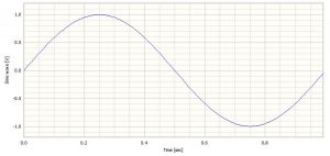
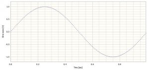
At first, the signal appears to be very smooth, but upon closer inspection, it is possible to see that actually it is 128 points joined together by straight lines. These points are shown in Figure 2.
We can see from this example that a sampling rate which is over 100 times greater than the signal frequency gives us a reasonably good visual representation of the signal.
Time Domain or Frequency Domain Analysis?
The time domain is probably the easiest to understand. This is where we view data in respect to time. Most people will usually view a captured data waveform first in the time domain. So our independent axis is time.
Advertisement
COMPLEXITY MADE SIMPLE
From sensors to DAQ to analysis & reporting, Prosig supports your entire measurement chain
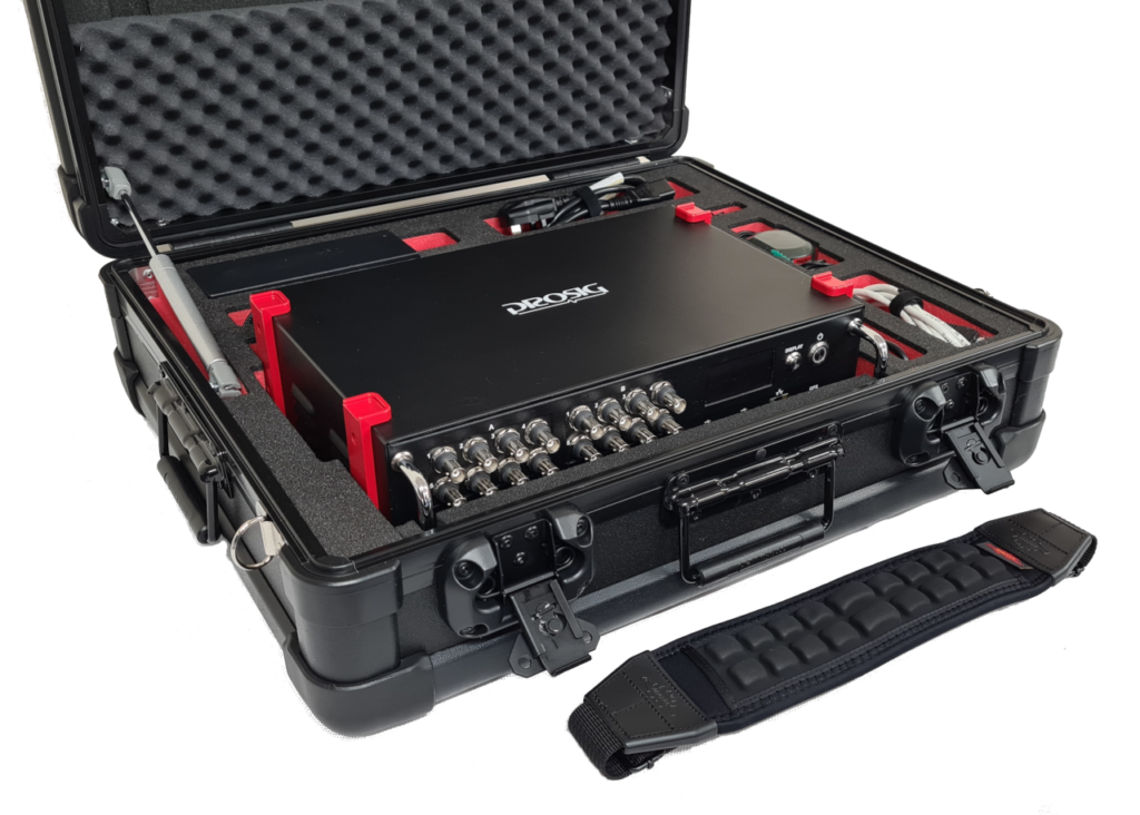


Whether you need accelerometers from our colleagues at DJB Instruments, microphones, pressure sensors or something else, Prosig can supply them as part of your system. Or you can use your own. Discover more about the Prosig hardware and software range.
The frequency domain is simply another way of viewing the same data, but in this case we look at the frequency content of the data. Now our independent axis is frequency, usually in Hertz (Hz). The Fourier Transform (FFT) is the most common analysis to take time domain data and create frequency domain data.
The following figure shows the signal from Figure 1 in the frequency domain as the result of an FFT transform.
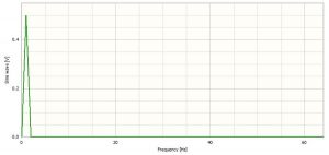
Note the range of the data on the x-axis in Figure 3. The data goes from 0 to 64 Hz, which is half the sample rate discussed previously. This is no coincidence and is carefully selected by DATS. The frequency which corresponds to half the sampling rate is known as the Nyquist Rate.
[Note also that the amplitude is 0.5, exactly half the amplitude of the signal in Figure 1. This half amplitude is an effect of the type of frequency transform that has been used. The exact reasons for this are outside of the scope of this article.]
What is the Nyquist rate?
The Nyquist rate, created from research by Harry Nyquist, is the sampling rate at which you have to sample a signal in order to capture all the frequency content of interest.
How does the Nyquist rate apply?
Note the peak at 1 Hz in Figure 3 and recall that this was the frequency of our original sinewave.
As we stated above, the Nyquist rate is the sample rate required to fully capture the frequency content of the signal. In our example above, the sample rate of 128 samples/second, or 128Hz, is more than enough to capture our 1Hz frequency content.
Say that we have a sinewave of 50Hz. Nyquist theory states that we would need to sample this signal at least 100Hz in order for the 50Hz to be fully represented. However, that is the very minimum required. Generally, in the real world, a factor of at least 2.5 is used. Some will even go as high as 4 to allow an adequate margin. It will depend on your application.
What happens if we ignore the Nyquist rate?
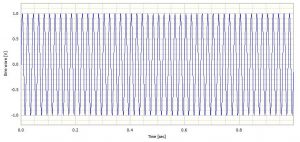
Figure 4 shows a 50Hz sinewave in the time domain, sampled at 2000 samples per second. Ignoring pixelation from the screen we can see a well defined sinewave.
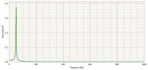
Figure 5 shows a 50Hz sinewave in the frequency domain, sampled at 2000 samples per second. Again, we can see a well formed peak at 50Hz as we would expect.
The same 50Hz sinewave in the time domain, sampled at 125 samples per second is seen in Figure 6. This is 2.5 x 50Hz, the minimum practical sample rate to capture the frequency.
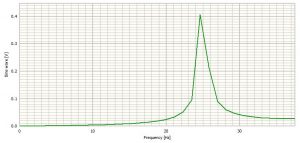
A 50Hz sinewave in the frequency domain, sampled at 125 samples per second is also shown in Figure 7.


Some degeneration of the signal can now be seen in the time domain. The frequency domain still looks acceptable as the peak is still around 50Hz. However, note the loss in magnitude of the peak in the frequency domain.
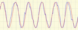
Figure 8 shows the 50Hz sinewave again but now sampled at 75 samples per second. This is below the minimum required to successfully represent the original signal. In Figure 9 the same data is shown in the frequency domain.

As you can see, the time domain display no longer looks like the original signal. However, it could easily be assumed to be plausible from a quick cursory look and without prior knowledge of the signal content.
The frequency domain no longer contains the information we expect. The frequency domain graph suggests a sine wave of 25Hz. The cause of the erroneous reading is a phenomenon called aliasing. The sample rate is no longer enough to successfully represent the original signal.
The concept of the Nyquist rate and aliasing are equally important when we consider resampling the data by downsampling.
Downsampling
The idea of downsampling is remove samples from the signal, whilst maintaining its length with respect to time.
For example, a time signal of 10 seconds length, with a sample rate of 1024Hz or samples per second will have 10 x 1024 or 10240 samples.
This signal may have valid frequency content up to 512Hz or half the sample rate as we discussed above.
If it was downsampled to 512Hz then the frequency content would now be reduced to 256Hz, due to the Nyquist theory. However, if there were frequencies present in the original signal between 256 and 512Hz they would be subject to aliasing and would cause incorrect frequencies to be displayed in the frequency domain.
So, in order to downsample the signal we must first low pass filter the data to remove the content between 256Hz and 512Hz before it can be resampled.
Upsampling
The purpose of upsampling is to add samples to a signal, whilst maintaining its length with respect to time.
Consider again a time signal of 10 seconds length with a sample rate of 1024Hz or samples per second that will have 10 x 1024 or 10240 samples. As above, this signal may have valid frequency content up to 512Hz, half the sample rate.
The frequency content would not be changed if the data was upsampled to 2048Hz. No content has been added to the signal so there would be no aliasing issues. The effect of upsampling is to improve resolution in the frequency domain.
NOTE if a signal is under-sampled initially and is subject to aliasing, upsampling will not resolve this.
Further Reading
We have looked at how we can upsample and downsample and the considerations we need to make with regard to Nyquist. Here is some further reading:
How Do I Downsample Data?
by Dr Colin Mercer, June 2001
Interpolation Versus Resampling To Increase The Sample Rate
by Dr Colin Mercer, June 2009
Aliasing, Orders and Wagon Wheels
by Dr Colin Mercer, June 2010
James Wren
Latest posts by James Wren (see all)
- What Are dB, Noise Floor & Dynamic Range? - January 12, 2024
- How Do I Upsample and Downsample My Data? - January 27, 2017
- What Are Vibration, Torsional Vibration & Shaft Twist? - November 8, 2016


Very useful article
Thank you for your comment. Your feedback is appreciated.
This article helped me understand the topic better, thank you! I do have one question though.
You mention in this article that “The idea of downsampling is remove samples from the signal, whilst maintaining its length with respect to time.”
At first I thought that when resampling a signal you change its duration, for example if you downsample a signal it get “compressed” aka has shorter duration. Running the example of decimate that matlab gives, I noticed that the duration of the downsampled signal is shorter (from 100s to 30s). I am still confused about what happens to the duration of a signal when resampling, because I’ve come across both cases on the internet and both kind of make sense.
Any clarification on the topic would be very helpful. 🙂
Hello Mark,
Thank you for your comments.
Lets assume you are discussing a time domain signal.
If you were to down sample the signal it’s length in time will not be changed. That is the number of seconds the signal is long stays the same.
It would have less samples per second but the number of seconds duration remains the same. And if you were to up sample a time domain signal the number of seconds remains the same but the number of samples per second is increased.
If you have experimented in your mentioned software and after down sampling the software shows a different duration then something is incorrect.