A common requirement to measure overall level vibration (or noise) as a function of time. Now, the overall level is a measure of the total dynamic energy in the signal. That is it does not contain the energy due to the DC level, which is the same as the mean value. The overall level is often loosely referred to as the signal RMS value. However the formal definition of the RMS level is that it contains the DC level as well as the dynamic energy level. If only the dynamic contribution is required then the measure needed is, strictly speaking, the Standard Deviation (SD). Sometimes it is useful to refer to the SD as the Dynamic RMS.
An analogy is that the DC level (mean value) is a measure of the Potential Energy, the Standard Deviation is a measure of the Kinetic Energy and the RMS value is a measure of the Total Energy. In mathematical terms then:
RMS2 = DC2 + SD2
Obviously if the signal already has zero mean or it is reduced to zero mean then the DC part is zero and both the SD and RMS will be identical.
Another common source of confusion between the Overall Level and the Dynamic RMS (SD) value is that the Overall Level is usually expressed in dB’s whilst the Dynamic RMS is generally given as a level in terms of the measurement units. For instance the Overall Level of an audio signal might be given as 94dB. As the dB reference level for audio signals is 2*10-5 Pascals this is the same as saying it has a Dynamic RMS of 1.0024 Pascals, which for practical purposes is 1 Pascal.
There are several ways that the dynamic rms or overall level may be evaluated in the DATS software package. One of the simplest and most effective is to use the trend analysis options. There are two trend options that are applicable, namely RMS and Standard Deviation. Normally the Standard Deviation option is the appropriate one as in noise and vibration work only the dynamic energy is of interest.
The Trend Evaluation analyses generally have three parameters. The first two parameters are ‘Integration Length’ and ‘Output Interval Step’. The third parameter, Independent Style, allows a choice of either ‘Independent Units’ or ‘Points’ and this governs how the first two parameters are interpreted. If you choose ‘Independent Units’ and we are dealing with a time history, then the first two parameters are specified in terms of seconds. Typically for a sound or vibration signal a suitable integration time is 0.5 seconds and the interval size would be say every 0.1 seconds.
Using these values the module calculates the overall level over the first 0.5 seconds, that is from 0.0 seconds to 0.5 seconds. It then advances 0.1 seconds and calculates the overall level from 0.1 to 0.6 seconds. This then repeats until we reach the end of the signal. This scheme is often called ‘hopping’ as the software hops along from section to section.
The critical parameter to select is the ‘Integration Length’. Setting this too long will smooth out any temporal changes and having it too short will not smooth enough! A good way of selecting the integration time is to think what frequency resolution would be typical if doing a frequency analysis on the signal. Then recall that integration time and frequency resolution are inversely proportional. That is if the appropriate frequency resolution is say 5Hz then the integration time is 1/5 = 0.2 seconds.
Selecting the ‘Output Interval Step’ is usually quite simple. Typically if the integration time is T seconds then using T/5 is a good starting choice.
As an example consider the typical engine runup signal shown below. This was analysed using Evaluate Trend (Standard Deviation) with a 0.5 second integration time and a 0.1 second interval step. The results are shown below, first on a separate graph with a dB scale and then as an overlay on the original time history.


Dr Colin Mercer
Latest posts by Dr Colin Mercer (see all)
- Data Smoothing : RC Filtering And Exponential Averaging - January 30, 2024
- Measure Vibration – Should we use Acceleration, Velocity or Displacement? - July 4, 2023
- Is That Tone Significant? – The Prominence Ratio - September 18, 2013