Aliasing, Orders and Wagon Wheels

These days most people collecting engineering and scientific data digitally have heard of and know of the implications of the sample rate and the highest observable frequency in order to avoid aliasing. For those people who are perhaps unfamiliar with the phenomenon of aliasing then an Appendix is included below which illustrates the phenomenon.

In saying that most people are aware of the relationship concerning sample rate and aliasing this generally means they are aware of it when dealing with constant time step sampling where digital values are measured at equal increments of time. There is far less familiarity with the relevant relationship when dealing with orders, where an order is a multiple of the rotational rate of the shaft. For example second order is a rate that is exactly twice the current rotational speed of the shaft. What we are considering here then is the relationship between the rate at which we collect data from a rotating shaft and the highest order to avoid aliasing.

The relationship depends on how we do our sampling as we could sample at constant time steps (equi-time step sampling), or at equal angles spaced around the shaft (equi-angular or synchronous sampling). We will consider both of these but first let us recall the relationship for regular equi-time step sampling and the highest frequency permissible to avoid aliasing. This is often known as Shannons Theorem [Learn more about Claude E Shannon].

Standard Aliasing

With regular time based sampling using uniform time steps we have a sample rate of say S samples/second. That is digital values are taken 1/S seconds apart. For convenience let $\delta T$ be the time increment in seconds so that $\delta T = (1/S)$ seconds.

With regular time domain processing we have a time and frequency relationship. That is if we carry out a Fourier analysis of a regularly spaced time history then we get a frequency spectrum.

Shannon’s aliasing theorem states that if we have a sample rate S then the highest frequency we can observe without aliasing is (S/2) Hz. (S /2) is known as the Nyquist Frequency. As previously mentioned the implication and results of aliasing are illustrated in an appendix below.

So if we have a time step $\delta T$ then the highest frequency, $f_{max}$ , is given by

$f_{max} = \frac{1}{2\delta T} = \frac{sample\,rate}{2} = \frac{S}{2} Hz$

This is a relationship between time steps in seconds and the highest frequency in Hz. It is worth noting that originally frequencies were specified in units of “cycles per second”, and that the fundamental units of Hz are 1/second.

Highest order with time based sampling

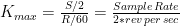
First recall that orders are multiples of the rotation speed of the shaft. So if a shaft is rotating at R rpm (revs/minute), then the Nth order corresponds to a rotational rate of (N*R) rpm. So if a shaft is notating at 1000 rpm then second order is 2000 rpm but if the shaft rotation speed was 1500 rpm then second order corresponds to a speed of 3000 rpm. Orders are independent of the actual shaft speed, they are some multiple or fraction of the current rotational speed.

The relationship between order and frequency for a given basic rotation speed of R rpm is simply:

$1^{st}order = R rpm = R/60 revs/sec = R/60 cycles/sec = R/60 Hz$ $K^{th}order = KR rpm = KR/60 revs/sec = KR/60 cycles/sec = KR/60 Hz$

Putting this relationship into the regular time based relationship to find the highest order to avoid aliasing gives:

$K*(R/60)=S/2$

That is the highest order, $K_{max}$ , when using time based sampling at S samples/second is given by:

$K_{max} = \frac{S/2}{R/60} = \frac{Sample\,Rate}{2 * rev\,per\,sec}$

Synchronous or Equiangular Sampling

With equiangular sampling we take N points per revolution, typically by using a toothed wheel or similar to give exactly N points per revolution. This is again independent of the actual shaft speed. So our sample rate is N points/revolution.

With equiangular sampling we are in the “revolution” domain and the corresponding domain is the order domain. That is if we carry out a Fourier analysis of an equiangular spaced signal then we get an order spectrum.

Applying the Shannon Theorem directly we have quite simply the result that with synchronous sampling where we have a sample rate of N points per revolution then our highest order to avoid aliasing, $O_{max}$ , is given by

$O_{max} = N/2$

Incidentally if we Fourier analyse over an exact number of revolutions, say P revs, then our order spacing is 1/P orders.

Spatial Sampling

Just for completeness the same applies if we do spatial sampling by measuring at equally spaced distance increments. The corresponding domain is wave number. Thus if we sample a road surface at L points per metre then our highest wave number to avoid aliasing, $w_{max}$ , is given by

$w_{max} = L/2$

Why use synchronous sampling?

With high-speed data acquisition systems it is quite usual to be able to sample at 100K samples/second. So if we are dealing with a shaft speed of say 6000 rpm, which is 100 revs/sec, then the highest order is [100000/ (2×100)] = 500. With synchronous sampling we would need an encoder with 1000 points/rev to achieve the same level. Often we are not interested in such high orders and there is rarely any high order content. That means we can use lower time based sample rates or lower points per revolution. So what is the advantage?

The essential point is that when we transform a synchronously sampled signal we are taken directly into the order domain. If we have sampled data covering exactly B revolutions then our order spacing will be (1/B) orders. Further the measurements at each order will be exact as they are precisely centred at each order.

If we have a time based signal those are two approaches. One way is to use waterfall analysis and the other is to convert the data to synchronously sampled data by software. Both of these methods require the tachometer signal to be captured at the same time. The accuracy depends upon precisely locating the tacho edges. The problem is illustrated below. Suppose the blue coloured signal is the actual tacho signal and the green one is the digitally sampled tacho. Now the * on the measured signal (green) are the actual data points. The actual tacho goes between a low of zero and a high of unity. So suppose we set the tacho crossing level at 0.6 and use the first data point that occurs at or above the threshold level on a rising edge as determining the actual tacho crossing point. This will directly lead to time jitter, adding and subtracting from each period. This will appear as noise and possibly as false frequencies.

Clearly the software could improve the situation, for example in DATS the software uses an interpolation process to determine a better estimate of the time location of the crossing point.

With waterfalls the next step is to determine a speed curve and then to carry out Fourier analysis at appropriate speed steps. The orders are then extracted from those frequency points which are the closest to the actual order being extracted. This is yet another approximation. An improved amplitude estimate is to determine the rms value over a short interval in the frequency domain. As one can see from the very description of the stages there exists considerable room for errors in the final order estimate.

When converting to synchronous sampling again it is essential to determine the tacho edge accurately. The next step is to interpolate the amplitude. This in theory can be done precisely by using a {(sin x) /x} basis but it requires signals and integrations of infinite length. In practice a reasonable estimate can be achieved with a relatively small number of points by using the most appropriate interpolation technique, such as a Lagrange based method.

Synchronous sampling avoids these complications.

Appendix -Aliasing Demonstrations

One of the classical demonstrations of aliasing is the so called “wagon wheel effect” where in films as the stage coach goes faster the wheels appear to go slower ad then to go backwards. If you would like to see a visual demonstration of the wagon wheel effect then the link below is excellent.

Initially the spokes rotate anticlockwise then slow and begin to rotate clockwise. What is particularly nice in this presentation is that there are other ‘markers’ at a smaller angular spacing that remain in the “non-aliased” region. Thus one can see parts of the wheel rotating and other parts stationary, most impressive and convincing. There are sliders that allow manual control of the wheel speed.

See Wagon-wheel effect from Michael’s “Optical Illusions & Visual Phenomena” (http://www.michaelbach.de/ot/mot-wagonWheel/index.html)

Another common form of illustrating aliasing is to show a high frequency sine wave sampled at too low a rate. If we sample too slowly we do not see the blue curve but rather we only see the data at the * points, which have been aliased to a much lower frequency.

For those of a mathematical leaning then we may find the apparent digital frequency from the following formula:

$f_d = |f_a - Kf_s|$

where $f_s$ is the sample rate, $f_a$ is the actual frequency, $f_d$ is the ‘digital’ frequency, and $K$ is the integer, starting from zero, such that $|f_a - Kf_s|$ is at its smallest.

We may write this as

$f_d = min_{k=0}^\infty | f_a - Kf_s|$

For example consider a sample rate of 500 samples per second and what happens to various frequencies.

Actual Frequency (f_a Hz)	Minimising K value	Alias frequency (f_d Hz)
180	0	180
280	1	220
380	1	120
480	1	20
580	1	80
680	1	180
780	2	220
880	2	120
980	2	20

Note how the pattern repeats.

Bio
Latest Posts

Dr Colin Mercer

Founder / Chief Signal Processing Analyst (Retired) at Prosig

Dr Colin Mercer was formerly at the Institute of Sound and Vibration Research (ISVR), University of Southampton where he founded the Data Analysis Centre. He then went on to found Prosig in 1977. Colin was MD and Chairman of Prosig for many years. He retired as Chief Signal Processing Analyst at Prosig in December 2016. He is a Chartered Engineer and a Fellow of the British Computer Society.