This article discusses quantifying basic vibration signals from three aspects: signal type, signal level, and signal display format. Mathematical expressions and typical applications are also introduced.
A simple harmonic vibration
A vibration whose displacement is a harmonic function of time is called a simple harmonic vibration, the simplest and most basic vibration.
For example, a sinusoidal wave can be expressed mathematically as
Displacement:

where 

For this sinusoidal displacement signal, its velocity and acceleration are related mathematically by a function of frequency, amplitude and time, as shown in Figure 1 and by the following equations:
Velocity:

Acceleration: 

The velocity and acceleration are the 1st and 2nd order differentiation of the displacement of the original sinusoidal wave. The phases are shifted by and amplitudes are multiplied by in sequence. Theoretically, it doesn’t matter which quantity is measured as the other two can be derived from the measured one. However, in some cases, the result obtained by performing integration or differentiation for the actual measured signals is not necessarily as ideal as in theory. Special care shall be taken. Generally, although displacement, velocity and acceleration can be converted to each other by differentiation and integration, direct measurement is always recommended.
The reasons causing this inaccuracy can vary. See Ref[1], Ref[2] and Ref[3] below for previous blog posts which explain this in detail.
Basic Vibration Signals – Choosing the correct signal type
Choosing a suitable parameter provides convenience for quantifying the vibration severity. Therefore, the physical mechanism behind the vibration shall also be considered. In basic vibration signals, displacement directly reflects the distance travelled, velocity represents the vibration energy, and acceleration is associated with the acting force. The differences between these different types of signals are discussed below.
Considering a signal may contain wide-range frequency components, displacement measurement usually gives a better interpretation of low-frequency components. In contrast, acceleration measurement gives the high-frequency components the most weight. Displacement measurement is mostly used when relative position change is of great interest. For example, to evaluate a shaft vibration, the displacement of the rotating shaft is always concerned at the shaft’s fundamental frequency, where the maximum amplitude appears. The clearance between rotor tips and casing measurement to investigate blade rubbing is another typical displacement application. A detailed application about displacement measurement is introduced in this article Ref[4].
Advertisement
Some examples of the products from the CMTG brands
DJB Accelerometers
Sense

- Piezoelectric charge & IEPE accelerometers
- Instrumentation, cables & accessories
- Calibration & repair service

Prosig DATS Hardware
Capture
- Rugged, mobile data capture
- Options inc. 24-bits @ 300k samples/sec
- From 4 to 1000’s channels

Prosig DATS Software
Analyze

- Don’t just test – gain insight from your data
- Huge selection of signal processing algorithms
- Optional application add-ons
In practice, acceleration is widely used for most general vibration measurements mainly due to the wide availability, size and lower cost of accelerometers. Acceleration is defined as the rate of change of velocity which correlates to energy in the system. Non-zero acceleration indicates that external force or energy is added to the system. Comparing the expressions of the displacement and acceleration for the above simple sinusoidal wave and ignoring the phase shift, the amplitude of acceleration is 
Velocity measurement is often used for mid-frequency range vibration. A likely explanation is that a given velocity level corresponds to a given energy level, so that vibration at low and high-frequency ranges are equally weighted from a vibration energy point of view. In industry, the velocity level is widely accepted to give a good indication of vibration severity on machine vibration in the mid-frequency band, 50 – 5KHz.
Quantifying the vibration level
Amplitude is the most intuitive quantity of basic vibration signals and reflects the vibration levels in both time and frequency domains. Vibration amplitude can be quantified via different metrics, which have different definitions. The most frequently used definitions include, for example, peak-to-peak level, zero-to-peak level, and the Root-Mean-Square (RMS) level. The peak-to-peak and zero-to-peak levels are mostly used to detect a transient vibration/shock. In contrast, the RMS level is a statistical value and is usually used to evaluate the vibration severity over a certain period of time.
Figure 2 compares different definitions used to quantify a signal level
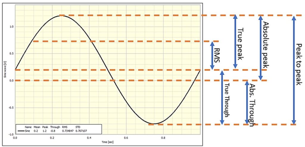
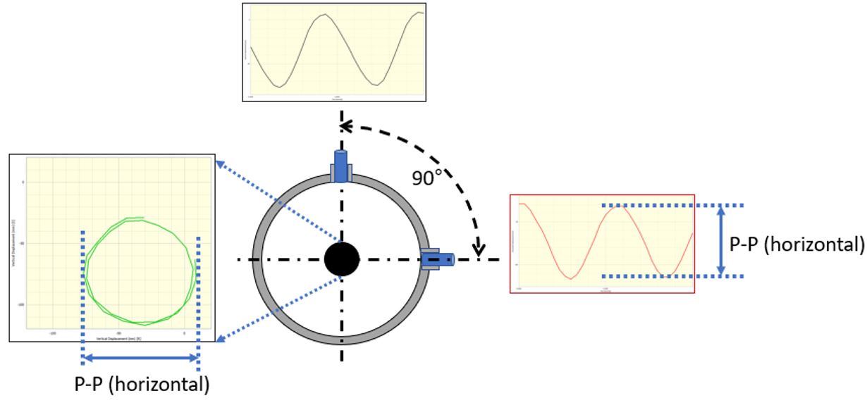
The peak-to-peak level is the relative value between a peak and a through. As a peak has “direction” towards maximum (peak) or towards minimum (through). The premise to evaluate this value is that the vibration is supposed to be “balanced” or vibrating around its mean. Therefore, the peak–to–peak value can either indicate a state of “imbalance” or envelope the trajectory of a movement. For example, Figure 3 shows a setup to measure the movement of a shaft that shall rotate around the shaft centre. Two proximity probes are installed in the vertical and horizontal directions, 90° apart. The peak-to-peak value marked in Figure 3 represents the change in the gap between the shaft centre to the probe for a complete revolution of the shaft. This value is usually separated into its AC and DC components associated with the movement of the rotating shaft about its centre and the distance from the average distance from the shaft to the probe, respectively. The orbit graph shown on the left corner displays the gap size changing when the shaft is rotating, which is widely used to monitor shaft vibration in rotating machinery. The details of this rotating shaft monitoring can be found in Ref[4].
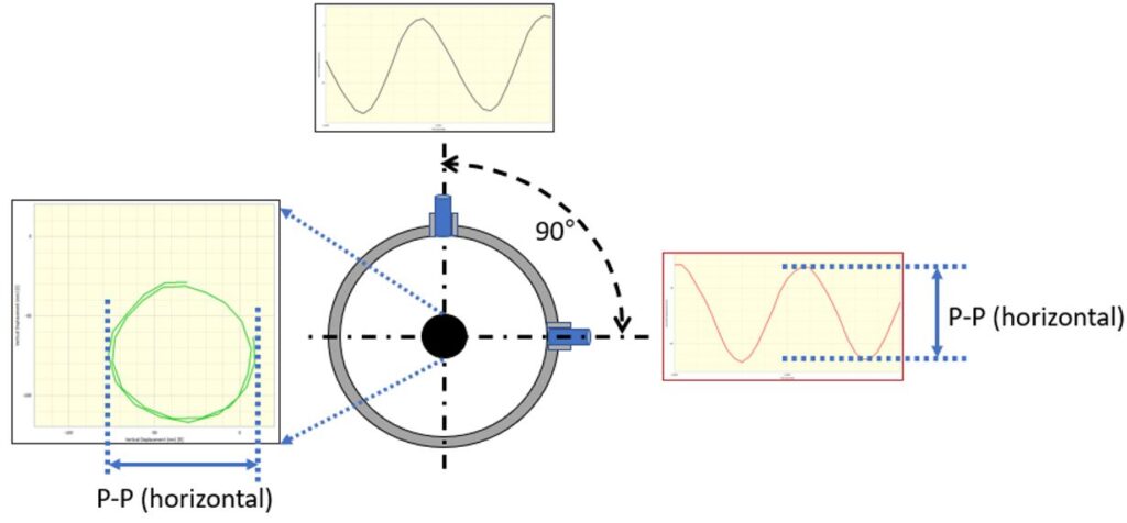
In Prosig’s DATS software, the peak-to-peak value can be calculated using the maximum difference between the positive-slope peak and negative-slope peak of a periodic waveform within any user-defined cycle.
Zero-to-peak is normally defined as half of the peak-to-peak value, also called “true peak” by some software. This value is the offset of the vibration away from the “equilibrium” state. If the measured quantity is velocity, zero-to-peak corresponds to the maximum dynamic energy of the motion, which is an important indicator of the severity of vibration.
It is worth noting that, for peak-to-peak and zero-to-peak, the sampling rate used or filters applied may influence whether the peaks can be captured accurately. Special care shall be taken.
Another important metric is the RMS value which is mathematically defined as
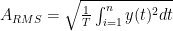
Here T is the over which the RMS calculation is performed, and y(t) is the time history of any type of vibration. For a Sine/Cosine wave, the RMS value is 
Generally, when people talk about an overall level of vibration, they refer to RMS level; this should be reflected in the units shown, i.e. mm/s RMS. Please note it is recommended to check if the Overall level includes any static or DC component.
For example, If v(t) contains both the potential energy (DC level) and kinetic energy (AC level), the RMS value corresponds to the total energy of the motion. And the overall dynamic energy shall use the standard deviation (SD), with the definition as:
![SD = \sqrt{\frac{1}{T}\int_0^T [v(t)-\overline{v(t)}]^2 dt}](https://s0.wp.com/latex.php?latex=SD+%3D+%5Csqrt%7B%5Cfrac%7B1%7D%7BT%7D%5Cint_0%5ET+%5Bv%28t%29-%5Coverline%7Bv%28t%29%7D%5D%5E2+dt%7D&bg=ffffff&fg=000&s=0&c=20201002)
For a stationary signal, as shown in Figure 4, its statistical properties are time-invariant, absolute RMS and dynamic RMS has the following relation:

If this stationary signal has zero mean, absolute RMS and dynamic RMS are equal as DC is zero. Therefore, this is no confusion when using the RMS value to represent the overall level.
Dr. Colin Mercer gave a detailed explanation about when RMS values contain a DC component in Ref[5]
When the signal is non-stationary, a simple case is shown in Figure 5. This signal is a random signal with a linearly increasing mean. Its SD doesn’t change with time but RMS has a similar trend as to the mean.

Users should be careful about how the overall level is defined in different software, especially for the situations and applications discussed above.
In general, when capturing data from velocity or acceleration sensors, most acquisition systems introduce AC coupling filters to remove any DC component. This is especially true when using ‘constant current’ or IEPE sensors where the AC component represents the vibration measurement which sits on top of the sensor compliance voltage.
Basic Vibration Signals – Display formats of vibration level
To review and analyse a vibration signal, a graphical representation of how the signal changes with respect to time, frequency, speed, etc. is the most intuitive way. Choosing the most appropriate display format will help to identify the quantities concerned easily.
Generally, linear amplitude scale is the default option when plotting a signal. It is a true representation of the actual measured vibration amplitude. A signal plotted via a linear amplitude scale equally displays a constant factor changes for all levels. Linear amplitude scaling can make a large dynamic range easily identified, but very low amplitude may be neglected. For example, as shown in Figure 6, in the case of machine vibration, the spectrum is composed of the fundamental frequency of the shaft and its harmonics. The components in the highlighted region could be an important fault indicator in such parts as bearings which often begin with small-amplitude vibration over a high-frequency range as highlighted. These peaks with small amplitude cannot be easily identified on a linear scale, however, can be better observed by applying logarithmic scale on amplitude axis. A log scale is one in which the steps in spatial distance of the scale represent changes in powers of 10 (usually). Therefore, data is compressed to a much greater degree at the high end than it is at the low end, and it is this very property that makes it so good for visually representing data with a large dynamic range.
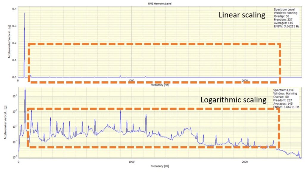
Logarithmic scaling of the x-axis is often used to plot power spectra whose energy covers a large frequency range. User shall choose a proper display format according to the data characteristics.
Make sure you don’t miss future posts. Sign up to our mailing list
Ref[1] Calculating Velocity or Displacement from Acceleration Time Histories
Ref[2] Converting Acceleration, Velocity and Displacement
Ref[3] Vibration: Measure Acceleration, Velocity or Displacement?
Ref[4] Shaft Displacement Measurement Using A PROTOR System
Ref[5] Time Varying Overall Level Vibration (or Noise)
Dr Cindy (Xin) Wang
Latest posts by Dr Cindy (Xin) Wang (see all)
- Prosig Shock Response Analysis - May 26, 2026
- DATS-HITS Using gfai tech Automatic Impact Hammer - March 4, 2026
- Impact Hammer Double Hit – An Investigation - June 13, 2023