This post discusses analyzing shaft twist and at the same time handling the less than perfect data that we have all come across.
A shaft has been instrumented with two shaft encoders, one at each end. Each shaft encoder gives out a once/rev pulse and a 720 pulses/rev signal. Each signal was digitised at 500,000 samples/second. The objective is to measure the twist in the shaft and analyze into orders. The test stand was already equipped with a data acquisition system so a Prosig acquisition system was not required. Instead it was decided that the data captured by the resident system would be imported into the DATS software. The only format available from the customer system was ‘comma separated variables’ or CSV. This is not ideal as it is an ASCII based format and therefore creates very large files.
To make the import as painless as possible it was automated using a DATS BASIC Script. Using DATS BASIC it was easy to create a function that asked the user to nominate a folder and then import all the CSV files it found into DATS. Once this had been done examination of the data could begin.
The graph in figure 1 shows a typical tacho plot, the particular example being the front trigger (once/rev) around 2.5 seconds into the acquisition.
At first sight all of the trigger signals look similar, with the obvious difference that the main tacho signals are 720 times faster.
A quick check on the validity or otherwise of the tacho signals is to generate speed curves, the results are shown in figure 2.
Clearly there is a problem with the front once/rev pulse. It one examines this around the 8 second region then the problem is clear as illustrated in figure 3.
There are missing pulses. At high speeds the problem gets worse. Applying the ‘tacho repair’ function to the speed curve does extend the range further as shown in figure 4.
Before determining the twist it is instructive to examine the speed curves derived from the once/rev and the 720 pulses/rev signals. The graph in figure 5 shows the speed curves over a very short time. The once/rev speed is gently rising at what is a locally constant rate whilst the 720/rev speed is obviously fluctuating about this trend due to torsional vibration.
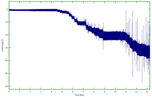
Calculating the twist angle uses a specific DATS module. The two signals used were the front and rear 720 pulses/rev signals. The result is shown in figure 6. Note the module also supports a gear ratio so it may be used through the valve train. The rear 720 pulse/rev signal was used as the reference. That is the twist is the front relative to the rear.
The first thing to note is that there cannot possibly be a 40 degree twist along the shaft. This is in fact caused by missing pulses and the like in the two pulse signals. This manifests itself as an abrupt “dc” shift in the twist versus time curve. Removing this from the twist curve is very simple, one just uses a suitable high pass filter on the twist signal. Given that the lowest speed is 6000 rpm then first order at that speed is 100 Hz. Thus using say a 5Hz High Pass filter will have no effect on anything below the 1/20th order.
A 5 Hz 96 dB per octave phaseless filter with a Butterworth amplitude characteristic was used. The result is shown in figure 7.
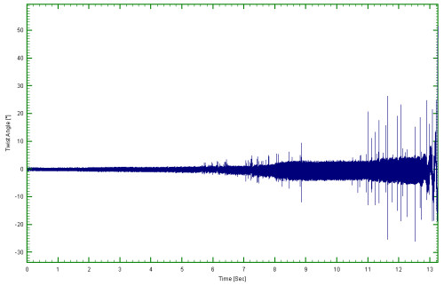
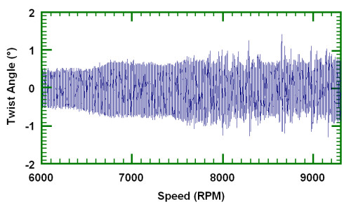
This has cleaned up the signal quite significantly. There are still some dubious extreme spikes. These are also due to tacho imperfections but their effect on a frequency analysis will be very small, basically they will raise the noise floor slightly. They appear as high frequency phenomenon. Of course as well as showing versus time we may also plot versus speed. An example is shown in figure 8 where we have also low pass filtered at 5kHz which removed most of the ‘spikes’.
Calculating the orders directly as a function of speed uses a specific DATS module, “synchronous orders versus speed”. This module uses a reference tachometer, in this case the once per rev rear trigger signal, to resample the data at constant angle separation. That is it internally generates the equivalent signal sampled at constant angles. The data is then Fourier transformed directly into the order domain. The following graph in figure 9 shows the first five orders in half order steps.

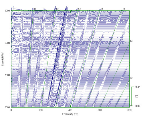
An alternative method is to construct a regular waterfall and then extract orders from that.
In this example the data was acquired at 500000 samples/second so we have a huge frequency range. This was necessary to get the twist signal which is essentially a differencing operation. We are, however, only interested in up to , say, 800Hz. Here the data was correctly decimated to give an effective sample rate of around 2500 samples/second.
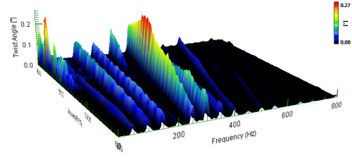
In figures 10 and 11 the data was decimated appropriately and then analyzed in 10 rpm steps. The data in the waterfall is only shown every 100 rpm for clarity, clearly there is little significant data after the fourth order.
Once the interactive analysis of the data was complete an automated solution was prepared for the customer. This consisted of two DATS BASIC Scripts. The first was used to take a folder name and convert all of the CSV data files in that folder into DATS datasets. A second script was then written that would take all of the datasets in a folder and perform the necessary twist and order analysis. This script then generated an Intaglio report for each test run.
In this way the customer could batch process a whole series of tests analyzing shaft twist with no further user intervention required. All they needed to do was collect the reports from the printer when they were complete!
Dr Colin Mercer
Latest posts by Dr Colin Mercer (see all)
- Data Smoothing : RC Filtering And Exponential Averaging - January 30, 2024
- Measure Vibration – Should we use Acceleration, Velocity or Displacement? - July 4, 2023
- Is That Tone Significant? – The Prominence Ratio - September 18, 2013


1. Based on the tacho signal in Figure 1, we can only calculate the speed at equi-spaced angular positions. How can the equi-spaced angular speed be processed to a RPM-Time signal in Figure 2? Is the speed curve in Figure 2 at equi-spaced time intervals?
2. Similar question for Figure 6 twist angle signal, is it at equi-spaced time intervals as well? Is it the result of front_speed-time signal minus rear_speed-time signal?
3. I do not quite understand your mentioned “This module uses a reference tachometer, in this case the once per rev rear trigger signal, to resample the data at constant angle separation.” What does the “data” for resampling refer to? Is it the data in Figure 1 or Figure 6?
Yes we can determine speed over 360 degree segments from the once per tacho pulse. But we can also refer those points to say the mid time points of the relevant tacho. This now gives an irregularly space speed versus time. This curve may in turn be interpolated using suitable algorithms into a speed versus equi spaced time increments. Here Figure 5 is the clue in that the once/rev speed is like the ‘average’ speed, and by looking over several revolutions in a moving frame one can obtain a reasonable estimate of the local ‘mean’ speed. At the same time we can get the angle travelled as a function of time in the same way. By using this it is then feasible to obtain speed as a function of angle
The multi-pulse/rev tacho is the local torsional velocity plus the mean local velocity. By suitably subtracting the calculated local mean velocity we are left with the torsional velocity, which in turn can be converted into torsional displacement.
The whole process is best described as angular or synchronous sampling.