With shafts, gears and the like, the general method of determining the rotational speed is to use some form of tachometer or shaft encoder. These give out a pulse at regular angular intervals. It we have N pulses per rev then obviously we have a pulse every (360/N) degrees. Determining the speed is nominally very simple: just measure the time between successive pulses. If this period is T_k seconds and the angle travelled is (360/ N) degrees then the rotational speed is simply estimated by 360/(N*T_k) degrees/second or 60/(N*T_k) rpm.

The above expression does not give the true speed as there will be measurement error in the period. If there is any torsional vibration then the effects of this will also be included. That is the measured period, T_k, is represented by

T_k = T_s +T_v + T_e

Where T_s is due to the underlying rotational speed, T_v is due to any torsional vibration and T_e is due to measurement errors.

Shown below is a fragment of a typical tacho pulse stream, in this case taken from a flywheel with 113 pulses/rev whilst doing a runup.

Using the DATS module ‘Vibration from Tacho’ then gives us the vibration amplitude as shown below. As well as the vibration amplitude we may also determine the vibration velocity. The vibration velocity in this example is typically less than 2% of the rotational velocity.

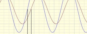
Incidentally if the velocity to displacement step is not carried out correctly then a curve such as show below could occur.

The above shape is unexpected and is clearly not correct. The major changes in level come from localised mean level components. When used in its default mode these are automatically removed by the software and we would see the angular vibration as shown in the first graph.

Before continuing further let us remind ourselves about time domain aliasing. In time domain sampling if we sample at S samples/second then we know that our alias frequency (also known as the Nyquist frequency) is simply S/2 Hz. This means that if we have any frequencies greater then S/2 Hz then they will be “reflected” back into the region 0 to S/2 Hz. Suppose for example we sample at 1000 samples per second, our alias frequency is 500 Hz. Thus any energy at 700 Hz will be reflected back about 500 Hz and will appear at 300Hz (up to 500 Hz and then reflected back 200 Hz making the “distance” travelled 700 Hz). We could also get multiple “reflections”, for example 1300 Hz would also appear at 300 Hz after a double reflection (up to 500 Hz, back to 0 Hz and then up to 300 Hz).

In the rotational frame we are not dealing with frequency as such but rather with orders. These are multiples of the rotational speed. So if the shaft is rotating at R rpm then second order is simply 2*R rpm, order 3.5. is 3.5*R rpm, and so on. Now let us consider what we have done in getting the vibration amplitude. Basically we have measured the period between successive pulses. Clearly if we have K pulses in each revolution then our effective sample rate for calculating the angular vibration is K pulses/rev. In a completely analogous way to time sampling, when we sample at K samples/rev then aliasing will occur if we have any order information above K/2 orders.

With modern analogue low pass filters aliasing is readily handled for time domain sampling. But when we generate the K periods per revolution we are effectively carrying out equi-angular sampling; which is a form of spatial sampling. The problem here is that there are no spatial anti alias filters. The mere action of creating the periods from the tacho causes aliasing. We cannot at that stage filter it out! Of course if there is no energy above the order alias value then that does not matter. We will return to this later.

Having determined the angular vibration signal it is natural to want to see this expressed in orders. To aid this, the ‘vibration from tacho’ module optionally creates an average speed signal such as shown below.

In this case it is a simple run up. As we have a speed versus time curve then we may generate a classical waterfall plot or extract any required orders. A typical set of extracted orders are shown below. We have not identified the individual orders below but we will return to that aspect later.

The corresponding waterfall plot showing the orders of most interest is given below.

At first-sight the waterfall plot seems fine. But notice that at some shaft speeds there appear to be some extra noise across the frequency spectrum. Now the above waterfall plot is only shown up to 200Hz, which is approximately up to about sixth order at the highest speed. The data was sampled at 12000 samples /second so expanding the frequency axis shows as below.

We can now see much more clearly the source of the interference.

Plotting against orders on the horizontal axis rather than frequency shows that the reflection point is at 56.5 orders, so we have spatial aliasing! Actually it is even more dramatic if we plot the waterfall of the vibration velocity.

Clearly there appears to be a single spatial alias incident that is causing multiple reflections. The Source seems to be located at around 1800 rpm and 56.5 orders. Now with that knowledge let us look again at the orders. This time we have also included the overall level, which is the level summed over all orders.

The overall shows an obvious spike at about 1800 rpm. It we look at the speed versus time curve this happens at around the 35 second mark which is where the speed signal shows a glitch. More subtle effects occur where this aliased data reflects. The waterfall shows the alias reaching the orders below the tenth order at around 2100 rpm. Indeed if we look at say the third and higher orders then we can see an apparent rise in these low amplitude orders in the 2100 rpm region. Although the source of the aliased data is quite large at 56.5 orders, by the time it reaches the orders of interest then the effects are relatively small. This is because our orders of interest are well below the order alias value. Spatial aliasing is a reality; we should always look to see if we have a problem as there is no spatial anti alias filter to get us out of the problem. Of course if we only had a few pulses per rev then aliasing could be more serious. Averaging in a sliding fashion over a few pulses also helps eliminate the effects but may cause a small underestimation of amplitudes. Just for the sceptics we filtered the vibration amplitude signal at 120Hz. The equivalent waterfall is shown below.

There is now nothing shown above 120 Hz but the effects of the spatial aliasing are still evident. If this is all we were shown would we have recognised this as spatial aliasing? Or would we just think it is “noise”? Even worse would we try to associate it with some phenomena in the system we are analysing?

As a closing remark whilst we are able to estimate the torsional vibration from a single tacho signal doing this on two separate tacho signals does not allow us to determine the twist. For that there is another specific “Twist” module that considers both tacho’s simultaneously.

The following two tabs change content below.

• Bio
• Latest Posts

Dr Colin Mercer

Founder / Chief Signal Processing Analyst (Retired) at Prosig

Dr Colin Mercer was formerly at the Institute of Sound and Vibration Research (ISVR), University of Southampton where he founded the Data Analysis Centre. He then went on to found Prosig in 1977. Colin was MD and Chairman of Prosig for many years. He retired as Chief Signal Processing Analyst at Prosig in December 2016. He is a Chartered Engineer and a Fellow of the British Computer Society.

Latest posts by Dr Colin Mercer (see all)

• Data Smoothing : RC Filtering And Exponential Averaging - January 30, 2024
• Measure Vibration – Should we use Acceleration, Velocity or Displacement? - July 4, 2023
• Is That Tone Significant? – The Prominence Ratio - September 18, 2013