

What are RC Filtering and Exponential Averaging and how do they differ? The answer to the second part of the question is that they are the same process! If one comes from an electronics background then RC Filtering (or RC Smoothing) is the usual expression. On the other hand an approach based on time series statistics has the name Exponential Averaging, or to use the full name Exponential Weighted Moving Average. This is also variously known as EWMA or EMA.
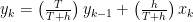
A key advantage of the method is the simplicity of the formula for computing the next output. It takes a fraction of the previous output and one minus this fraction times the current input. Algebraically at time k the smoothed output yk is given by

As shown later this simple formula emphasises recent events, smooths out high frequency variations and reveals long term trends. Note there are two forms of the exponential averaging equation, the one above and a variant

Both are correct. See the notes at end of the article for more details. In this discussion we will only use equation (1).
The above formula is sometimes written in the more limited fashion.

How is this formula derived and what is its interpretation? A key point is how do we select 
Now, an RC low pass filter is simply a series resistor R and a parallel capacitor C, as illustrated below.
The time series equation for this circuit is
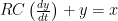
The product RC has units of time and is known as the time constant ,T , for the circuit. Suppose we represent the above equation in its digital form for a time series which has data taken every h seconds. We have

Rearranging gives
or

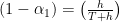
This is exactly the same form as the previous equation. Comparing the two relationships for a we have

which reduces to the very simple relationship

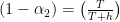
Hence the choice of N is guided by what time constant we chose. Now equation (1) may be recognised as a low pass filter and the time constant typifies the behaviour of the filter. To see the significance of the Time Constant we need to look at the frequency characteristic of this low pass RC filtering process. In its general form this is

Expressing in modulus and phase form we have
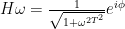
where the phase angle 

The frequency 

Clearly as the time constant T increases so then the cut off frequency 
It is important to note that the frequency response is expressed in radians/second. That is there is a factor of 

Actually, it is not the time constant we usually wish to select but those periods we wish to include. Suppose we have a signal where we wish to include features with a P second period. Now a period P is a frequency 


This gives some insight into how to set
By looking at the expansion of the algorithm we can see that it favours the most recent values, and also why it is referred to as exponential weighting. We have

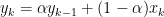
Substituting for yk-1 gives
![y_k = (1 - \alpha)x_k + \alpha\left[(1-\alpha)x_{k-1} + {\alpha}y_{k-2}\right]<br /> =(1 - \alpha)(x_k + {\alpha}x_{k-1}) + \alpha_2y_{k-2}](https://s0.wp.com/latex.php?latex=y_k+%3D+%281+-+%5Calpha%29x_k+%2B+%5Calpha%5Cleft%5B%281-%5Calpha%29x_%7Bk-1%7D+%2B+%7B%5Calpha%7Dy_%7Bk-2%7D%5Cright%5D%3Cbr+%2F%3E+%3D%281+-+%5Calpha%29%28x_k+%2B+%7B%5Calpha%7Dx_%7Bk-1%7D%29+%2B+%5Calpha_2y_%7Bk-2%7D&bg=ffffff&fg=000&s=0&c=20201002)
Repeating this process several times leads to

Because 
In summary, we see that the simple formula
- emphasises recent events
- smoothes out high frequency (short period) events
- reveals long term trends
Appendix 1 – RC Filtering – Alternate forms of the equation
Caution There are two forms of the exponential averaging equation that appear in the literature. Both are correct and equivalent.
The first form as shown above is 
The alternate form is 
Note the use of 

Earlier

which gives
Now choosing to define

gives
Hence the alternate form of the exponential averaging equation is

where

In physical terms it means that the choice of form one uses depends on how one wants to think of either taking 
The first form is slightly less cumbersome in showing the RC filtering relationship, and leads to a simpler understanding in filter terms.
[Original 28th April 2003]
[Updated 12th March 2013]
[Updated 30th January 2024]


Excellent! Exactly what I was looking for.
I think you want to change the ‘p’ to the symbol for pi.
Marco, thank you for pointing that out. I think this is one of our older articles that has been transferred from an old word processing document. Obviously, the editor (me!) failed to spot that the pi had not been transcribed correctly. It will be corrected shortly.
it’s a very good article explanation about the exponential averaging!
I believe there is an error in the formula for T. It should be T = h*(N-1), not T = (N-1)/h.
Mike, thanks for spotting that. I have just checked back to Dr Mercer’s original technical note in our archive and it seems that there was error made when transferring the equations to the blog. We will correct the post. Thank you for letting us know
Thank you thank you thank you. You could read 100 DSP texts without finding anything saying that an exponential averaging filter is the equivalent of an R-C filter.
Pingback: » Filtering Noise from Sensor Readings: A Simple Low Pass Filter The Aspiring Roboticist
hmm, do you have the equation for an EMA filter correct? is it not Yk = aXk + (1-a)Yk-1; rather than Yk = aYk-1 + (1-a)Xk
Alan,
Both forms of the equation appear in the literature, and both forms are correct as I will show below. The point you make is important one because using the alternate form means that the physical relationship with an RC filter is less apparent, moreover the interpretation of the meaning of a shown in the article is not appropriate for the alternate form.
First let us show both forms are correct. The form of the equation that I have used is
[latex]y_k = {\alpha}_1y_{k-1} + (1 - {\alpha}_1)x_k[/latex] …(1)
and the alternate form which does appear in many texts is
[latex]y_k = {{\alpha}_2}x_k + (1 - {\alpha}_2)y_{k-1}[/latex] …(2)
Note in the above I have used [latex]{\alpha}_1[/latex] in the first equation and [latex]{\alpha}_2[/latex] in the second equation. The equality of both forms of the equation is shown mathematically below taking simple steps at a time. What is not the same is the value used for [latex]{\alpha}[/latex] in each equation.
In both forms [latex]{\alpha}[/latex] is a value between zero and unity. First rewrite equation (1) replacing [latex]{\alpha}_1[/latex] by [latex]{\beta}[/latex]. This gives
[latex]y_k = {\beta}y_{k-1} + (1 - \beta)x_k[/latex] …(1A)
Now define [latex]\beta = (1 - {\alpha}_2)[/latex] and so we also have [latex]{\alpha}_2 = (1 - \beta)[/latex]. Substituting these into equation (1A) gives
[latex]y_k = (1 - {\alpha}_2)y_{k-1} + {\alpha}_2x_k[/latex] …(1B)
And finally re-arranging gives
[latex]y_k = {\alpha}_{2}x_k + (1 - {\alpha}_2)y_{k-1}[/latex] …(1C)
This equation is identical to the alternate form given in equation (2).
Put more simply [latex]{\alpha}_2 = (1 - {\alpha}_1)[/latex].
In physical terms it means that the choice of form one uses depends on how one wants to think of either taking [latex]\alpha[/latex] as the feed back fraction [equation (1)] or as the fraction of the input [equation (2)].
As mentioned above I have used the first form as it is slightly less cumbersome in showing the RC filter relationship, and leads to simpler understanding in filter terms.
However omitting the above is, in my view, a deficiency in the article as other people could make an incorrect inference so a revised version will appear soon.
Colin
I’ve always wondered about this, thanks for describing it so clearly.
I think another reason the first formulation is nice is alpha maps to ‘smoothness’: a higher choice of alpha means a ‘more smooth’ output.
Michael
Thanks for observation – I will add to the article something on those lines as it is always better in my view to relate to physical aspects.
Dr Mercer,
Excellent article, thank you. I have a question regarding the time constant when used with an rms detector as in a sound level meter that you refer to in the article.
If I use your equations to model an exponential filter with Time Constant 125ms and use an input step signal, I do indeed get an output that, after 125ms, is 63.2% of the final value.
However, if I square the input signal and put this through the filter, then I see that I need to double the time constant in order for the signal to reach 63.2% of its final value in 125ms.
Can you let me know if this is expected.
Many thanks.
Ian
Ian,
If you square a signal like a sine wave then basically you are doubling the frequency of its fundamental as well as introducing lots of other frequencies. Because the frequency has in effect been doubled then it is being ‘reduced’ by a greater amount by the low pass filter. In consequence it takes longer to reach the same amplitude.
The squaring operation is a non linear operation so I do not think it will always double precisely in all cases but it will tend to double if we have a dominant low frequency. Also note that the differential of a squared signal is twice the differential of the “un-squared” signal.
I suspect you might be trying to get a form of mean square smoothing, which is perfectly fine and valid. It might be better to apply the filter and then square as you know the effective cutoff. But if all you have is the squared signal then using a factor of 2 to modify your filter alpha value will approximately get you back to the original cut off frequency, or putting it a bit simpler define your cutoff frequency at twice the original.
Thanks for your response Dr Mercer. My question was really trying to get at what is actually done in an rms detector of a sound level meter. If the time constant is set for ‘fast’ (125ms) I would have thought that intuitively you would expect a sinusoidal input signal to produce an output of 63.2% of its final value after 125ms, but since the signal is being squared before it gets to the ‘mean’ detection, it will actually take twice as long as you explained.
The principle objective of the article is to show the equivalence of RC filtering and exponential averaging. If we are discussing the integration time equivalent to a true rectangular integrator then you are correct that there is a factor of two involved. Basically if we have a true rectangular integrator that integrates for Ti seconds the the equivalent RC integator time to achieve the same result is 2RC seconds. Ti is different from the RC ‘time constant’ T which is RC. Thus if we have a ‘Fast’ time constant of 125 msec, that is RC = 125 msec then that is equivalent to a true integration time of 250 msec
Dr Mercer,
Thank you for the article, it was very helpful. There are some recent papers in neuroscience that use a combination of EMA filters (short-windowed EMA – long-windowed EMA) as a band-pass filter for real time signal analysis. I would like to apply them, but I am struggling with the window sizes different research groups have used and its correspondence with the cutoff frequency.
Let’s say I want to keep all the frequencies below 0.5Hz (aprox) and that I acquire 10 samples/ second. This means that fp =0.5Hz; P= 2s; T = P/10=0.2;
h= 1/fs=0.1;
if:
T/(T+h)=((N-1)/N),
(T/h) + 1 = N
0.2/0.1 + 1 = N
N=3
Thefore, the window size I should be using should be N=3. Is this reasoning correct?
Before answering your question I must comment on the use of two high pass filters to form a band pass filter. Presumably they operate as two separate streams, so one result is the content from say [latex]f_{low}[/latex] to half sample rate and the other is the content from say [latex]f_{high}[/latex] to half sample rate. If all that is being done is the difference in mean square levels as indicating the power in the band from [latex]f_{low}[/latex] to [latex]f_{high}[/latex] then it may be reasonable if the two cut off frequencies are sufficiently far apart but I expect that the people using this technique are trying to simulate a narrower band filter. In my view that would be unreliable for serious work, and would be a source of concern.
Just for reference a band pass filter is a combination of a low frequency High Pass filter to remove the low frequencies and a high frequency Low pass filter to remove the high frequencies.
There is of course a low pass form of an RC filter, and hence a corresponding EMA. Perhaps though my judgement is being overcritical without knowing all the facts! So could you please send me some references to the studies you mentioned so I may critique as appropriate. Maybe they are using a low pass as well as a high pass filter.
Now turning to your actual question about how to determine N for a given target cut-off frequency I think it is best to use the basic equation T=(N-1)h. The discussion about periods was aimed at giving people a feel of what was going on. So please see the derivation below.
We have the relationships [latex]T=(N-1)h[/latex] and [latex]T=1/2{\pi}{f_c}[/latex] where [latex]f_c[/latex] is the notional cut-off frequency and h is the time between samples, Clearly [latex]h = 1/{f_s}[/latex] where [latex]f_s[/latex] is the sample rate in samples/sec.
Rearranging T=(N-1)h into a suitable form to include the cut-off frequency, [latex]f_c[/latex] and the sample rate, [latex]f_s[/latex], is shown below.
[latex]N=1+\frac{T}{h}=1+\frac{1}{2{\pi}{f_c}h}=1+\frac{1}{2{\pi}(\frac{f_c}{f_s})}[/latex]
So using [latex]f_c = 0.5Hz[/latex] and [latex]f_s = 10[/latex] samples/sec so that [latex](fc/fs) = 0.05[/latex] gives
[latex]N=1+\frac{1}{2{\pi}*0.05}=4.1831[/latex]
So the closest integer value is 4. Re-arranging the above we have
[latex]f_c = \frac{f_s}{2{\pi}(N-1)}[/latex]
So with N=4 we have [latex]f_c = 0.5307 Hz[/latex]. Using N=3 gives an [latex]f_c[/latex] of 0.318 Hz. Note with N=1 we have a complete copy with no filtering.
Could you restore missed images?
Thank you for spotting the missing images. They have now been restored.
What is N?
Where does the following formula come from?
y[k] = (N-1)/N * y[k-1] + 1/N * x[k]
Many thanks