
In one of our recent articles a question was asked regarding the practical use of real & imaginary type plots compared with modulus & phase type plots.
In general, noise or vibration signals are composed of one or more sinusoidal signals which can be quantified in terms of their magnitude (modulus) and phase components. These can be visualised as the result of a spectral transformation in the form of either a real & imaginary plot or a modulus & phase plot. The moduli & phases are directly related to the real & imaginary components. Real & imaginary is one way to visualise a complex number, modulus & phase is another way.
A sinusoidal vibration will have a magnitude which is the amount it is moving up and down. The phase component of the same signal is how much this sinusoid is delayed (in terms of an angle) compared with a reference sinusoid moving with the same frequency. This is an important point; the phase is only relevant if it is relative to a reference.
Say, for example, a simple, floating (free-free) beam has some form of sinusoidal excitation applied to one end of the beam and accelerometers are used to measure the responses at both ends. When both the phases are the same (at the excitation position and the response position) the ends of the beam will be moving up and down together as shown in Figures 1 and 2.


But when both the phases are not the same, the ends of the beam will be moving up and down at different times and the beam will pitch from side to side, as shown in Figures 3 and 4.


Now, to return to the original question, specifically about real & imaginary numbers:
A Real & Imaginary pair of numbers defines the position of the end point of a straight line drawn from the origin (0,0) of a two dimensional plot; one of the dimensions is the horizontal (real) part and the other dimension is the vertical (imaginary) part. This is known as rectangular complex data.

Real & imaginary data can also be expressed in the form of a pair of modulus & phase numbers, this is also known as polar complex. In this form the modulus is the distance from the origin and the phase is the angle that the line makes with the horizontal axis.

Essentially they are two different representations of the same data. Figures 7 and 8 show a frequency spectrum first in rectangular complex form and then in polar complex form respectively.

The output of a Fast Fourier Transform (FFT) analysis of a time signal is a spectrum of complex (real & imaginary) numbers. However, the human mind better understands and can visualise more easily a complex frequency spectrum when the data is displayed in the form of a modulus & phase plot as shown in Figure 8.

The same complex data can also be shown in two other ways: either by plotting the real spectrum versus the imaginary spectrum or the modulus spectrum versus the phase spectrum. This type of plot is commonly known as a Nyquist plot as shown in Figure 9 below. This combines the magnitude (modulus) and angle (phase) information into a single plot.

The data at each point of Nyquist plot corresponds to the complex amplitude at a particular frequency. Usually the data being displayed would be some sort of frequency response function which depicts how the response at a particular point varies in both amplitude and phase with changing frequency.
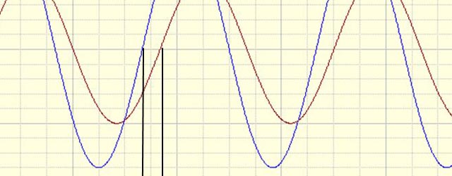
If a flexible structure is excited by a sinusoidal input force then in general the response in the time domain at any position will not be in phase with the excitation as shown in Figure 10 below.

From the time histories of the Excitation and Response the delay between the two signals can clearly be seen as both a time shift and a phase angle shift. In mathematical terms the response 


The frequency response at all frequencies from zero to half the sampling rate can be represented by a modulus spectrum of 

Normally, in noise and vibration work, we would use the modulus & phase form of presenting data. So what is the practical application of using the real & imaginary form? A good example would be modal analysis. Modal resonances usually appear as circles when a Frequency Response Function (FRF) is plotted in real versus imaginary form or as clearly defined peaks when the FRF is plotted as a modulus spectrum. However, in some situations when there are two or more resonance frequencies close together the two peaks can merge into a single peak thereby giving the impression that there is just a single modal resonance when in fact there are multiple resonances. By viewing an FRF as a Nyquist plot it is often easier to discern the presence of additional modes.
In our experience the modulus & phase form of display is by far the most widely used, and often the phase is not displayed at all. There are, however, cases where a real versus imaginary type of display shows phenomena that may be missed by the modulus & phase type of display.
Adrian Lincoln
Latest posts by Adrian Lincoln (see all)
- Averaging Frequency Response Functions From A Structure - June 17, 2016
- Seismic Qualification Testing (Part 1) - June 14, 2016
- What is Operating Deflection Shape (ODS) Analysis? - September 1, 2014


“In our experience the modulus & phase form of display is by far the most widely used, and often the phase is not displayed at all.”
Agree.
The phase may be important in experimental modal analysis while using two or more accelerometers. In particular, the phase difference can describe the vibration mode if the modulus measurements are similar.
“There are, however, cases where a real versus imaginary type of display shows phenomena that may be missed by the modulus & phase type of display.”
Such cases should be rare. The real physical information is given the modulus and phase.
Hello Adrian,
Can you explain in detail how to read the Nyquist plot.
One common application for the magnitude and phase approach is balancing airplane propellers and helicopter rotors. Where, of course, the only frequency of interest is the fundamental frequency of rotation. Everything above this threshold is typically filtered out.
I’ve had a great deal of difficulty in finding learning material on the web, describing this balancing process, and the attendant DFT process for identifying the magnitude and location of the “heavy spot”.
Can you recommend a source of information, for the layman, of the basic process and technology used in balancing such rotating machinery?
Honestly, dude, if you do not understand that concept you should be kept very far away from all important machinery.
(leave it to smart people to do)
My personal experience is that the best approach to understand the FRFs is to go back to the basics. The FRF can show displacement, velocity and acceleration. They are all related but shifted in phase. Whether to watch imaginary part or real part depends what you are using and what are you expecting from the analysis. But if you forget the analysis itself and go back to mathematics and the basic rules and reasons for usage of the complex numbers in analysis then everything will be clear.
Regarding Prasad’s question of Nyqvist plot (which I generally don’t use other than in teaching the basics) I really recommend the following book: ISBN-13: 978-0470746448
Anders Brandt, Noise and Vibration Analysis: Signal Analysis and Experimental Procedures
I need help with procedures where a linear system is connected to non-linear. The linear system is defined by its FRF and the non-linear is assumed to be SDOF with non-linear spring and viscous damper as well as frictional damping. Maybe I should mention that I work with silicone rubber based tuned mass dampers for automotive industry and experience Fletcher-Gent (amplitude dependency) effect in the rubber.
Philippe,
Thank you very much for the info.
Peter M
Honestly, dude, if you do not understand that concept you should be kept very far away from all important machinery. (leave it to smart people to do)
Peter, I’m sure your comment was intended to be tongue in cheek, but please remember that a lot of people come here to learn and we all have to start somewhere. I remember a time when even I wasn’t a genius. 🙂
wonderful explanations. thanks.
Can you explain real & imaginary axis concept by simulation
Hello balaji
There is a good explanation of complex numbers on Wikipedia here…
http://en.wikipedia.org/wiki/Complex_number
I hope that helps you.
is there any animation video clip of real & imaginary frequency
Hi balaji
Try using Google or another search engine to search for something like “complex numbers frequency animation”. You will find many results for what you are looking for.