Generating speed v time information from noise & vibration signals

Picture the scenario; you have captured some noise & vibration data from a rotating machine. Typically, this might be noise in a vehicle cabin, but could have been anything from a tiny pump to a full size power station turbine. So you have your data. Unfortunately, you didn’t manage to capture any information about the rotational speed. Maybe someone else was using the tacho sensor or the built-in speed sensor didn’t work. Perhaps there wasn’t time. Or, maybe, you just plain forgot. And, now, your boss wants some frequency v speed graphs and some order plots.

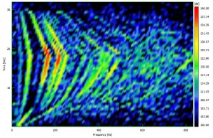
We all know that to analyze against speed we need speed information (see How To Measure Noise & Vibration In Rotating Machines and the accompanying video for more information). So, there isn’t much we can do with our data that has no speed information, is there? Well, that isn’t quite true. Luckily, DATS has a feature that can help out in these situations. Consider the following graph (Figure 1) of a frequency versus time plot. This is often called a “Hopping FFT” or “Short Time FFT”. This shows us the frequency spectra, in this case of vibration, varying over time. Time starts at the bottom of the graph and increases up the y-axis. Frequency is shown along the x-axis.

"Hopping FFT" of vibration signal — Figure 1: “Hopping FFT” of vibration signal

We can see from this plot that the frequency content of our data increases until just over half way through the measurement and then decreases again. From this we can infer that the test piece, in this case a vehicle engine, accelerated and then decelerated. We would normally refer to this as a “runup” and a “rundown”.

To enable us to extract a meaningful speed v time signal there are two things that it is helpful to know

what is the dominant order we would expect to see
approximately what was our maximum speed

The first of these is usually easy in the case of a four stroke engine or some similar machine. The reason for knowing this will become obvious in the following explanation of the techniques we are going to use. Knowing the maximum speed has a twofold purpose. First, it will enable us to verify our results and, second, the algorithm we are going to use can adapt itself and improve its accuracy using this information.

In our example we know that second order will be dominant since the data was taken from a 4-cylinder, 4-stroke engine. From simply observing the rev counter when we performed the test we know that the engine was revved to approximately 5000rpm. In Figure 2 we have added some lines and points that trace second order on the hopping FFT plot (click the graph to enlarge it).

Figure 2: Hopping FFT plot with second order trace added

If we were to read off the frequency and time for each of these points we would get a table something like that shown below.

Time (sec)	Frequency (Hz)
1.0	20
6.5	100
11.0	130
18.0	165
29.0	100
30.0	80

Now we know that the rotational speed of the fundamental frequency (first order) is given by multiplying the frequency by 60. For second order we multiply the frequency by 60 and divide by 2. For order n we can calculate the rotational speed using

$Speed\:in\:rpm = \frac{f*60}{n}$

where f is frequency in Hz.

If we apply this to our figures above we can obtain a table of time against speed.

Time (sec)	Speed (rpm)
1.0	600
6.5	3000
11.0	3900
18.0	4950
29.0	3000
30.0	2400

We have some degree of confidence in these figures since the maximum of 4900rpm is very close to our expected 5000rpm maximum.

Using this information we could use linear interpolation to generate more data points and make a reasonably accurate speed curve. Of course, we could trace and read off more points to improve the accuracy. This would allow us to perform some waterfall and order analysis with a fair degree of accuracy.

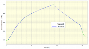
However, using the DATS Rotating Machinery Analysis software we can do even better than that. The software includes an interactive tool and a proprietary Adaptive Multi Dimensional Spectral Tracking Algorithm to closely track the orders contained in the noise or vibration signals to recreate an accurate speed v time signal. In Figure 3 below you can see a speed v time curve created using the algorithm compared to speed information recorded at the time of the test.

Figure 3: Calculated speed curve compared to measured speed curve

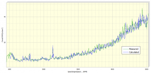
We then used the two speed curves to calculate the overall vibration level against rotational speed. The two results can be seen in Figure 4.

Figure 4: Overall level v speed using measured and calculated speed curves

It is plain that the results correspond very well. Obviously, the quality of results in these situations will vary with different data. For instance, vibration signals usually give better results than acoustic channels. Or, maybe, you don’t have one order that is dominant throughout the signal. However, the algorithm has been tested on some of the most difficult datasets we could find and there were very few cases that the Adaptive Tracking algorithm wouldn’t cope with.

If you would like to see more of the software I have made the following video which shows the software in action.

Bio
Latest Posts

Chris Mason

Chris' early love of computers & technology (Sinclair ZX80's, Commodore PETs & Apple ]['s) grew into a career in software development, product development, team leadership, web development, and marketing. He was General Manager at Prosig, part of CMTG, until June 2024. Chris graduated with an HND from Portsmouth Polytechnic and in 2019 completed an Executive MBA at the University of Winchester where he focused on innovation and strategy.